Abstract
The fundamental principles of optical holography for capturing the optical waves of physical objects, and its difference from photography, are described. A photograph can only record a single view of an object scene; a hologram is capable of capturing the entire optical wavefront that impinges on it. There should be little difference between observing a hologram and the physical object scene. Numerical generation of digital holograms, commonly known as computer-generated holography (CGH), is presented. Two important approaches in CGH, the point-based and the layer-based methods, are described. The point-based method is suitable for generating holograms of simple objects with a small number of object points; the layer-based method is preferred for an object scene with a large number of object points concentrated in a few depth planes. The method for recovering a 3-D scene image from a digital hologram is provided. Three different methods for capturing digital holograms of physical object scene are described. The first method is similar to the art of optical holography, but instead of a photographic film, a digital camera is used to record the holographic waves emitted from the scene. As a digital camera can only record intensity information, the method can only be employed to capture an off-axis, amplitude-only hologram. The other two methods, known as phase-shifting holography (PSH) and optical scanning holography (OSH), are capable of capturing both the magnitude and phase components of the holographic signals. PSH is faster in operation, while OSH can be used to capture holograms of large objects. A simplified version of OSH, known as non-diffractive optical scanning holography (ND-OSH), is presented. ND-OSH is similar in principle to OSH, but the complexity of the optical and electronic setups is reduced.
1.1 Basic Concept of Holography
When light impinges from one medium to another, part of it will be transmitted while the rest will bounce back to the environment or be absorbed into the medium. Figure 1.1(a) shows a ray of monochromatic light (i.e., single frequency or wavelength) L falling on a planar interface between two different homogeneous media M1 and M2.The beam is inclined at an angle θ1 with respect to the normal of the interface. Assuming that M2 is partially transmissive, and L is a plane wave, the direction of part of the light transmitting through M2 will be changed from θ1
 to θ2
to θ2 . This process is known as refraction, and the relation between the pair of angles is governed by Snell’s law.
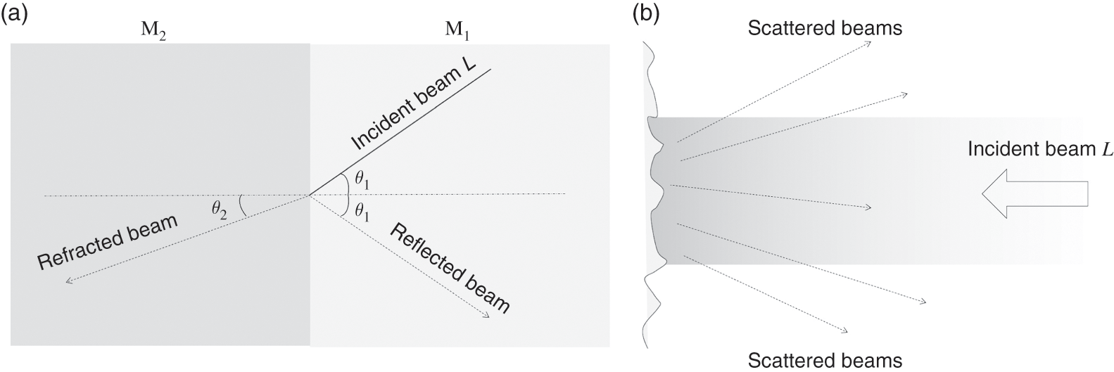
If the interface between the two media is smooth, the light that is not refracted will be reflected back as specular (mirror-like) reflection, in which case the angle of incident θ1 will be identical to the angle of reflection θ2
 . For an interface with a rough surface composed of microscopic irregularities, the incident beam will be scattered, resulting in diffusive reflection, as shown in Figure 1.1(b). Scattering is a generic term that refers to the change in the propagation path of an electromagnetic wave as it is intercepted by some form of non-uniformities in a medium. Optical scattering results when a beam of light hits one or more tiny particles.
The light impinging on a physical object undergoes one or more of the abovementioned modes of propagation. Light emitted from the illuminated object surface conveys information on the shape and color of the object. As the emitted light waves fall on the retina of human eyes, an image of the object will be perceived by the brain.
Photography and optical holography are methods for capturing the emitted light waves from an object scene onto a photographic film. When the photographic film carrying the recorded optical signals is presented to an observer, the light waves of the object scene will be partially or fully reproduced to the eyes of an observer. At present, there are two major approaches in capturing the light waves of an illuminated object: photography and holography. Photography is the art of capturing the part of the optical waves corresponding to a two-dimensional (2-D) projected view of an object, while holography captures the entire optical waves. A photograph only presents the intensity or color of a scene; it is a planar image and does not contain any disparity or depth information. With holography, all the light waves emitted by the object are captured, and hence are capable of reproducing a three-dimensional (3-D) view of the object. These two image-recording techniques are explained as follows.
Light, or optical signal, is a kind of electromagnetic wave in the form of a time-varying sinusoidal wave oscillating with a certain amplitude and frequency. When a person observes a scene, optical waves of different intensities and frequencies will be received by different groups of sensory cells in the retina, creating the impression of color and brightness. The instantaneous amplitude v(t) of a single beam of monochromatic light L is generally expressed as:
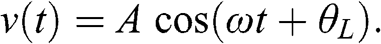 (1.1)
(1.1) In Eq. (1.1), t represents the time variable, while the terms ω
 and θL
 denote the frequency and phase of the light beam, respectively. For a monochromatic light wave of constant frequency, the frequency term is sometimes left out, and the representation of the wave can be simplified as v=Aexp(iθL)
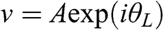 , where i denotes the imaginary unit. In the physical world, an object reflects an infinite number of light beams from its surface, and the collective excitation of these optical signals on the retina leads to the formation of an image of the object to an observer.
Next, we shall explore how the optical waves of an object can be captured. Imagine the light wave of an object, which is sometimes referred to as the object wave, is intercepted by a transparent medium that is capable of recording the amplitude and phase of every optical beam that passes through it, as shown in Figure 1.2(a). For the time being, let’s ignore the details of the mechanism behind the recording process. As this medium is illuminated by a coherent plane optical wave (i.e., the amplitude and phase at every part of the wavefront is identical), the light beam that emerges from every point on it will be modulated (in amplitude and phase), by an amount that is identical to that which has been recorded. As illustrated in Figure 1.2, the observer will see the same set of optical waves from either the object or the recording media. Theoretically, the optical waves received by the retina in both cases should be identical, hence casting an impression of the same image.
Figure 1.2 (a) Capturing object waves of an object on a recording medium. (b) Reconstructing a virtual object image from the recording medium with a coherent plane optical wave.
The magical recording media is known as a hologram, a word that finds its origin from the Greek words ὅλος (whole) and γραφή (drawing). Literally, the word hologram carries the meaning of something that is capable of recording the complete information of a visible image. Theoretically, there is little difference between looking at the virtual image of a hologram and the actual object. Hence, from a hologram, an observer should be able to see not only the color and intensity of the object, but also all the depth cues and disparity information. Depth cues are the visual information in an image that instigates the perception of distances between the observer and different parts of the object. For example, the lens of our eye will change its focus when objects at different distances are observed. Another example of depth cues is when the viewpoint of an observer is panned (shifted along a certain path): an object that is closer will appear to translate more than one that is farther away, which again creates the sensation of difference in depth between the objects. Disparity, sometimes referred as “binocular disparity,” is the deviation in the location of an object as observed by the left and the right eyes. Through the disparity, our brain is able to interpret the depth of different objects in the scene.
The art of capturing a hologram of an object is commonly referred to as optical holography. The method was invented in late 1940 by Dennis Gabor, who was awarded the Nobel Prize in Physics in 1971 for his contribution to the invention and development of the holographic method. Works of Gabor in optical holography were reported in [1], and later by Bragg in [2]. There have been numerous advancements in optical holography since, and a comprehensive description on the developments can be found in [3,4]. For completion, a brief outline of holography is given here.
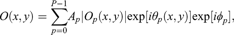
The concept of holography can be illustrated from a more analytical point of view. Figure 1.3 shows the side view of an object scene containing a single object point. The intensity of the object point is white, represented with a value of unity. A recording medium is positioned at the hologram plane to record the light wave of the object scene. As the white object point is illuminated with a coherent plane wave (i.e., a wavefront that is homogeneous in magnitude and phase), it will behave as an isotropic point light source that scatters an object wave O0(x,y) onto the hologram. Extending this concept, for a single object point with intensity A
 , the object wave O(x,y)
 that is projected on the hologram is given by
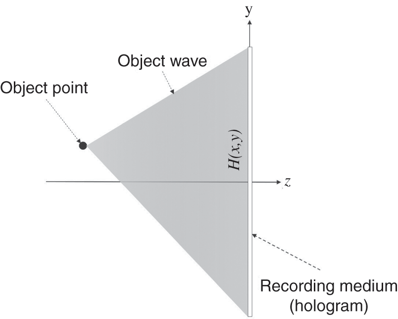
Figure 1.3 Object wave projected by an object point of unit intensity on the recording medium.
 (1.2)
(1.2) In Eq. (1.2), the magnitude and phase of the object wave of a point source are denoted by |O0(x,y) | and θ0(x,y)
 , respectively. The term ϕ0
 is the phase of the light illuminating the object point, which will be added to the phase component of the object wave.
The above principles of hologram formation can be easily applied to a scene with multiple object points. An arbitrary object surface can be considered as comprising many isotropic point sources, each emitting its own object wave when illuminated. The optical signal recorded on the hologram is the superposition of the optical wave emitted from each object point. The mixing of these waves is a process that is commonly known as optical interference:
 (1.3)
(1.3) where P is the total number of object points, and subscript p is the index of the object points. The object wave recorded on the hologram is referred as the interference pattern. For a coherent plane wave propagating along the axial direction (i.e., normal to the hologram plane), the phase ϕp of the illuminating wave is constant for all the object points, which can be ignored or included as a constant phase term in the computation of the object wave. If the illumination light beam is incoherent, the value of ϕp
 is random for different object points, and the object wave can no longer represent the light field of the source object.
For the time being, assume there are some means that enables the full object wave to be recorded on a medium, resulting in a hologram (denoted by the function H(x,y) in Figure 1.3). The signals on the hologram are complex-valued (with magnitude and phase components), and in the form of high-frequency fringe patterns. Different names have been adopted in various literatures to describe hologram signals, such as – but not limited to – fringe patterns, hologram fringes, diffractive waves, or holographic signals. These terms will be used throughout this book.
As shown in Figure 1.2(b), a coherent plane wave passing through a hologram is modulated, both in amplitude and phase to give the same object wave O(x,y) . From the reconstructed object wave, the observer will be able to see a realistic 3-D image of the object from the hologram. The process of recovering a 3-D image from the hologram is known as “reconstruction.” The use of a coherent optical plane wave is mandatory as it will not change the amplitude and phase of the object waves – that is, Ap
 and θp(x,y)
 of each object point in both the recording and the reconstruction processes.
1.2 Optical Recording in Practice
A conceptual optical setup for recording the hologram of an object scene is shown in Figure 1.4. The actual recording system is slightly more complicated. A thin laser beam is converted into a plane wave with the use of a beam expander (BX), and illuminates the specimen after passing through the semi-transparent beam splitter (BS). A laser beam is used because it is coherent, so the phase distribution of its wavefront is homogeneous. As explained in Section 1.1, it is necessary that the phase ϕp of the illumination beam on every point on the object surface is constant. The beam expander magnifies the cross-sectional area of the thin laser beam so that the illumination light will be wide enough to cover the entire object of interest. The object wave emitted by the object of interest is partially reflected by the beam splitter to the recording media. If both the amplitude and phase of the object wave can be captured, the recording medium, will become the hologram of the specimen. Unfortunately, this ideal scenario is difficult, if not impossible, to achieve in practice.
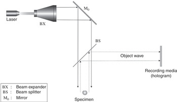
Figure 1.4 Conceptual optical setup in hologram recording.
The reason is that optical recording materials developed to date, commonly known as photographic films, are usually implemented with a layer of gelatin emulsion coated onto a plastic substrate. The emulsion comprises microscopic grains of silver halide crystal, each of which will be partially converted into silver upon exposure to light. Upon exposing the film to an optical image, the chemical property of each silver halide crystal will change proportionally to the intensity of light falling on it, forming an invisible or latent image. Subsequently, the film can be chemically developed into a visible image. Since the silver halide crystal is only responsive to the intensity of light, a photographic film is only capable of recording the intensity, but not the phase, of a light field. Instead of the full holographic information, the signal recorded on the photographic film is only constituted by the magnitude component of the object wave, as given by
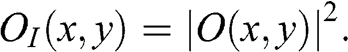 (1.4)
(1.4) Apparently, the signal recorded by the photographic film in Eq. (1.4) is different from the object wave, as it does not carry any information on the phase component. Due to the absence of the phase terms, an image of the specimen cannot be reconstructed from the signal OI(x,y) .
.
1.3 Photography
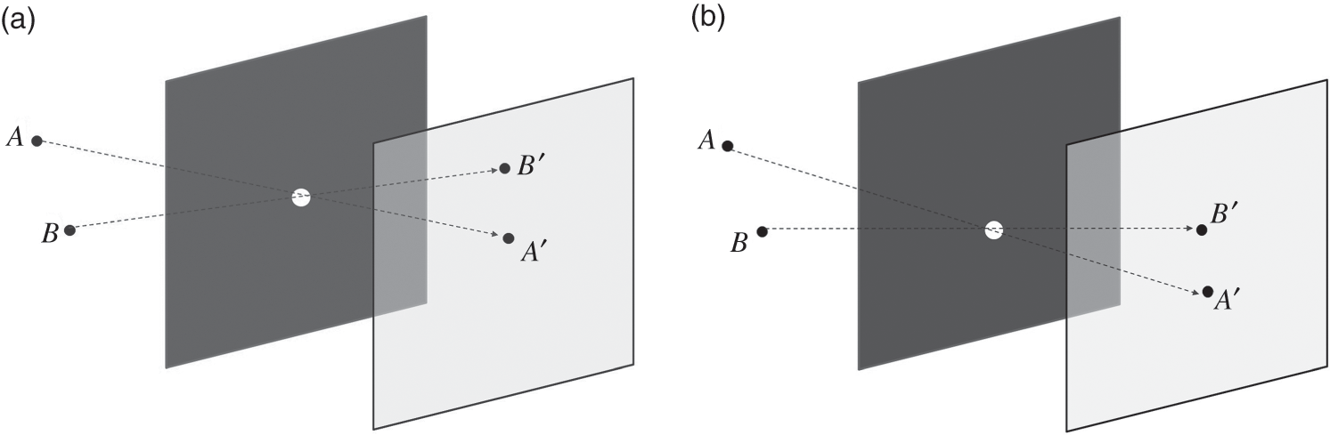
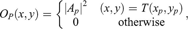
The classical art of photography can be interpreted as a special case of optical holography, although it was invented at a much earlier date when the art of holography was unknown to the world. As seen in Eq. (1.4), it is not possible to record the phase component of the object wave with a photographic film. Photography is based on capturing a small part of the object waves that carries the optical image of a specific viewpoint of the object scene. The concept is to place a small aperture between the object scene and the photographic film (a.k.a. a photograph), so that there is a one-to-one mapping between the light wave emitted from each object point and a single point on the recording plane. In another words, the light waves of different object points will not interfere with one another as they fall onto the recording media. Such an implementation is known as a “pinhole camera.” Figure 1.5(a) shows the imaging of a pair of point light sources, A and B, with a pinhole camera. The tiny pinhole only allows a light wave of a unique orientation for each object point to pass through, and impinges on an image plane at which a photographic film is placed. Restricted by the pinhole, each location on a photograph can only receive the object wave of a single object point. Mathematically, the magnitude of the object wave received by a photograph from a single object point at location (xp,yp) is expressed as
 (1.5)
(1.5) where T(xp,yp) denotes a one-to-one transformation on the coordinates (xp,yp)
 . From Eq. (1.5), the function OP(x,y)
 is simply a transformed image of the object scene, with the object point recorded at the position T(xp,yp)
 . On the image plane, the image of an object point is flipped horizontally and vertically, and relocated to a new position according to the location of the pinhole. Note that the object wave contains only the magnitude component (i.e., the intensity) of the light wave of a unique point source on the photograph. As a result, the phase component of the light wave is not involved in the recording process, and the object can be illuminated with incoherent light (e.g., ambient lighting from the sun and fluorescent lamps), whereby the phase of the illumination beam on each object point can be totally random and uncorrelated with each other.
The photograph can only capture an image of the object scene at a particular viewpoint that is constrained by the position of the pinhole. With a single view of the object scene, the recorded image cannot convey any depth cue or disparity information. To capture another viewpoint of the object scene, the position of the pinhole has to be changed. Figure 1.5(b) shows the imaging of the pair of object points, A and B, with the pinhole shifted to a different location. From these two figures, the images of the two object points are relocated to different positions on the recording plane.
1.4 Recording Setup in Optical Holography
Although holographic technology can be traced back to 1940, hologram recording was not practiced until the development of the laser in the 1960s, which is capable of generating a coherent light wave. As mentioned before, coherent illumination is mandatory in holographic recording. The first hologram was demonstrated in 1962 by the Soviet scientist Yuri Denisyuk [5], as well as by Emmett Leith and Juris Upatnieks of the University of Michigan in the USA [6]. Different to photography, optical holography records a 3-D – instead of 2-D – image of the object scene onto a photographic film by preserving both the amplitude and phase components of the object wave. Intuitively, this may sound a bit contradictory, as a photographic film is only responsive to the intensity of the light wave. In holographic recording, this problem is overcome by converting the complex-valued holographic signal into intensity information prior to recording on a photographic film. The conversion is achieved by adding the complex-valued object wave with an inclined reference plane wave, which is also derived from the coherent beam that illuminates the object. The result of adding the pair of waves is an interference pattern (which is also commonly referred to as a beat pattern), encapsulating both the magnitude and phase components of the object waves. A typical optical setup for recording an off-axis hologram is given in Figure 1.6.
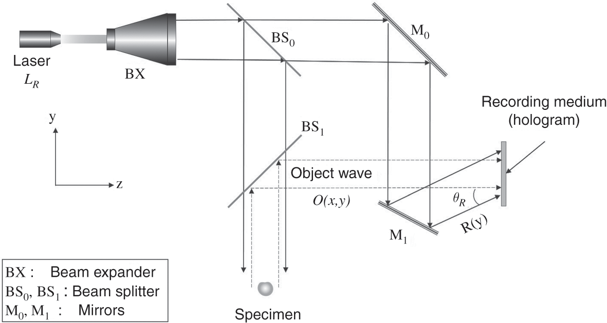
Figure 1.6 Practical optical setup for recording an off-axis hologram.
Similar to Figure 1.4, the source of illumination is a monochromatic laser beam LR which is expanded into a plane wave via a beam expander. The expanded beam is divided into two separate paths after passing through a beam splitter. The first beam is reflected by the beam splitter BS0, propagates through the beam splitter BS1, and illuminates the specimen. The object wave O(x,y) from the specimen is reflected by BS1, and impinges on the hologram. The second part of the expanded beam is reflected to the hologram via mirrors M0 and M1, projecting the beam onto the hologram at an angle of incidence θR
 along the vertical direction, resulting in an inclined reference plane wave
 (1.6)
(1.6) where λ is the wavelength of the laser beam. Note that R(y)
 is a pure phase function. If θR=0,
 the reference wave is simply the plane wave that is used to illuminate the specimen. When the object wave and the reference wave meet on the surface of the photographic film, they combine to form an interference pattern. The magnitude of the interference pattern is then recorded on the photographic film, resulting in a hologram with the intensity given by

where C1=[|O(x,y)|2+|R(y)|2] , C2= O(x,y)R*(y)
 , and C3=O*(x,y)R(y).
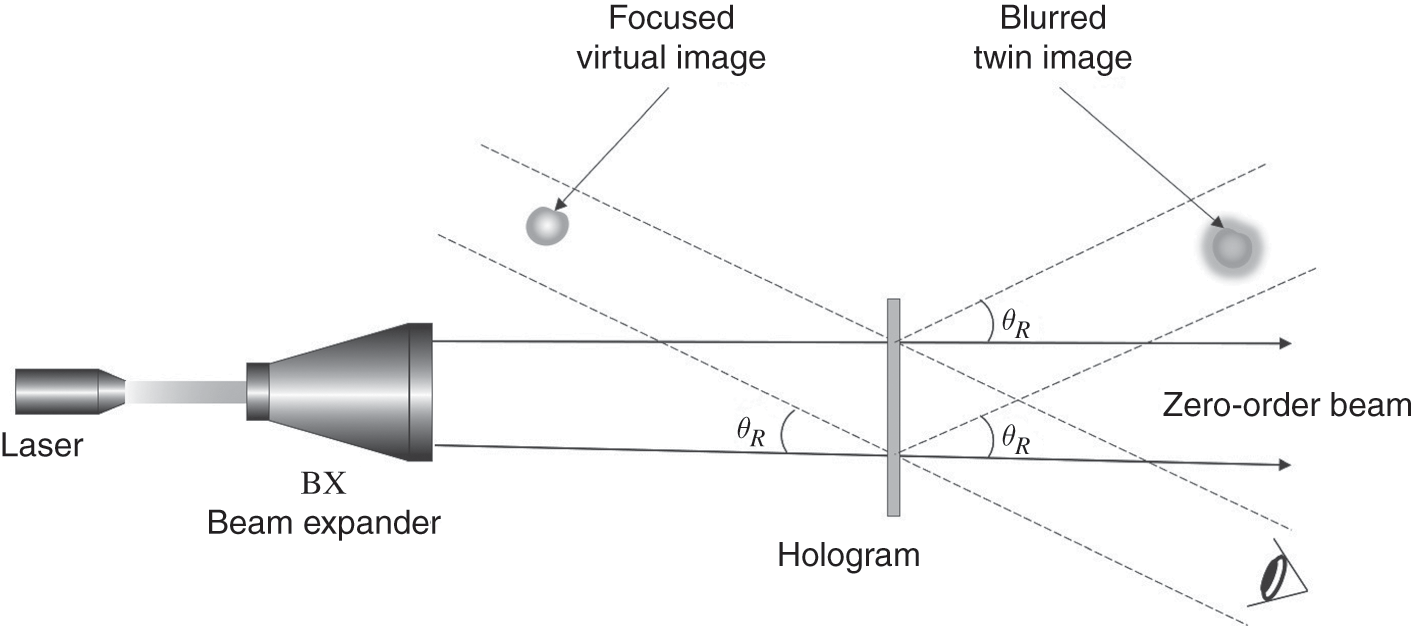
From Eq. (1.7), the hologram H(x,y) is a real signal that can be recorded onto the photographic film. Subsequently, the object wave can be optically reconstructed from the hologram by illuminating it with a plane wave, as shown in Figure 1.7. The light wave emitted by the hologram is contributed by three different components, each corresponding to a term in Eq. (1.7).
The first term C1 is the sum of the intensities of the object and the reference beams. Due to the absence of the phase component, this part of the light wave does not carry useful information on the 3-D image of the specimen, and appears as a patch of highlighted region. The second term C2
 is identical to the object wave apart from the constant phase term R*(y)
 , while the last term C3
 is the conjugate of the object wave multiplied with the reference wave R(y)
 . Being different from C1
 , the complex object wave of the specimen are encapsulated in both C2
 and C3
 .
.
From the optical wave of the illuminated hologram, three images can be observed. The first one is a focused, virtual image of the object scene that is reconstructed from the component C2 . This component of the optical wave contains the object wave O(x,y)
 in the hologram H(x,y)
 , with the addition of the phase term R*(y)
 . The virtual image can be viewed from an oblique angle, as shown in Figure 1.7. The second image is a blurred, defocused twin image corresponding to C3
 , which carries O*(x,y)
 , the conjugate of the object wave, and the phase term R(y)
 . Similar to the virtual image, the twin image can be observed from another oblique angle. The third image, usually referred to as the zero-order beam, is constituted from the remaining term C1
 , and can be observed from the axial direction. Apart from the virtual image, the other pair of images are unwanted content as they do not form a correct reconstruction of the object scene.
From Figure 1.7, it can be seen that mixing of the object wave O(x,y) with the inclined reference wave R(y)
 has imposed an angular separation θR
 between each consecutive pair of images that are reconstructed from the hologram. It can be inferred that if θR
 is small, the virtual image could be partially overlapping with, and hence contaminated by, the twin image and the zero-order beam. As such, the angular separation θR
 must be large enough that the virtual image can be separated from the unwanted content, and optically reconstructed as a standalone visible image. Even if this is achieved, there is still a good chance that all three components are visible to the observer, although they are not spatially overlapping with one another. This is one of the major disadvantages of an off-axis hologram.
Theoretically, the virtual image can be fully separated from the unwanted content by increasing the value of θR . In practice, due to the limited resolution of the photographic film, a ceiling on the angle θR
 is imposed. As explained previously, a photographic film comprises individual microscopic grains of photosensitive materials, each of which constitute a pixel on the film. The resolution of the photographic film, therefore, is limited by the size of the pixel. Assuming that all the pixels are square in shape and have identical size of δd×δd
 , an image recorded on it is effectively discretized with a 2-D sampling lattice with a sampling interval δd
 along the horizontal and vertical directions. According to sampling theory, this will impose an upper limit to the spatial frequency of the recorded signal.
To determine the maximum angle of incidence, consider a simple case where only the reference wave is present. For a given θR , the spatial frequency of the hologram fringe pattern is the minimum, as compared to the case when the object wave is present. Figure 1.8 shows the side view of a reference wave which is inclined at an angle θR
 along the vertical axis. As the signal on the hologram is discretized into pixels when it is recorded on the photographic film, the vertical axis is denoted by the variable n
 , where n
 is an integer representing the row indices of the pixels. The physical location of the kth row along the vertical axis is given by y=kδd
 . A pair of light beams of the reference wave is shown in Figure 1.8, impinging on the hologram at n=0
 and n=k.
 The relative phase difference between these two beams is given by
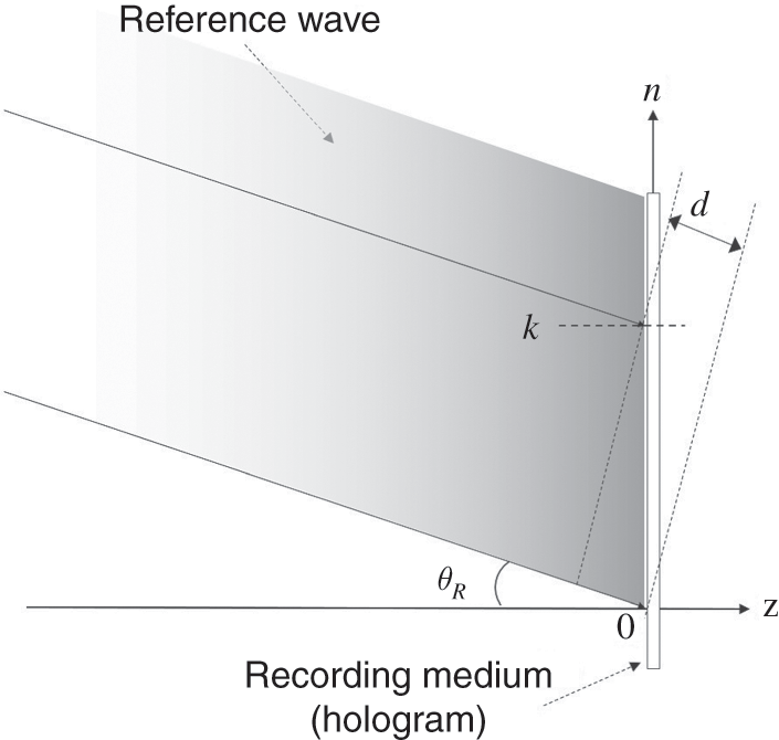
Figure 1.8 An inclined reference wave.
 (1.8)
(1.8) where ω=2πδdλ−1sin(θR) rad/s. From Eq. (1.8) it can be visualized that the fringe pattern on the hologram is a sinusoidal wave with frequency ω
 . As the maximum frequency that can be represented in the discrete signal is π
 rad/s,
 (1.9)
(1.9) For small value of θR , this expression can be approximated as
 (1.10)
 In Eq. (1.10), a hologram with pixel size of δd can only record an incline plane wave with a maximum angle of incidence θmax=0.5λδd−1
 . This implies that the maximum viewing angle of this hologram is also limited to the angle θmax
 .
.
A plot of the angle θmax versus the pixel size δd
 of the hologram is shown in Figure 1.9. It can be seen that θmax
 is inversely proportional to the pixel size of the hologram. Hence, the higher the resolution of the hologram, the larger will be the angular separation between the virtual image, the zero-order beam, and the twin image.
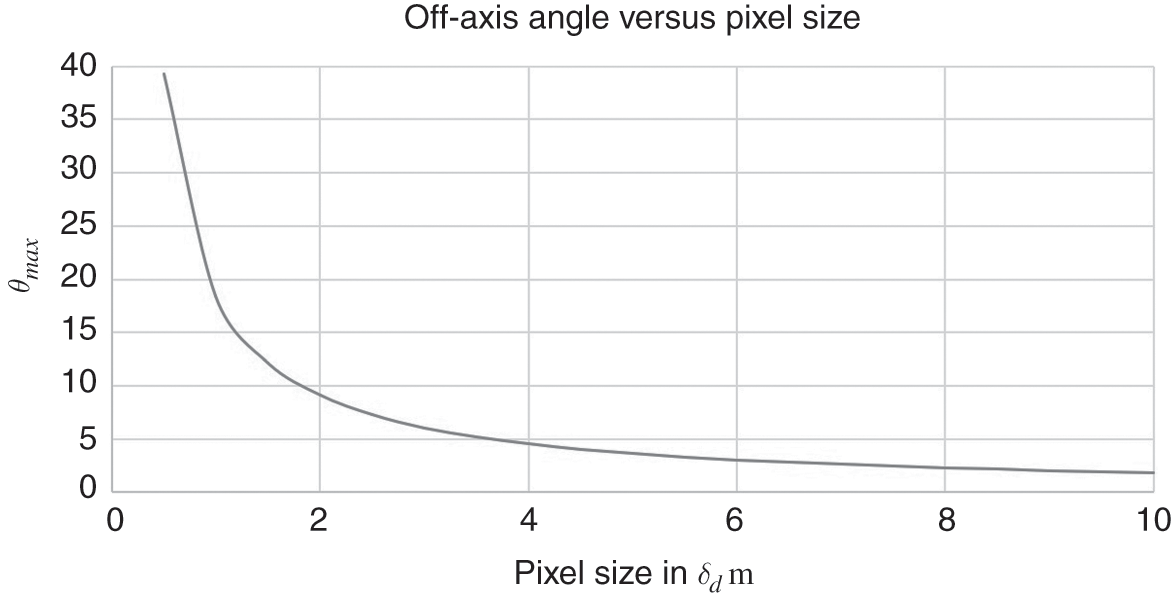
Figure 1.9 Plot of θmax versus pixel size of the hologram.
In optical holography, the hologram of a physical 3-D object is recorded in a photographic film. With the advancement of computing and electronics technologies, a digital hologram can be generated numerically from a computer graphic model, or captured from a physical object scene with a digital camera. In the following part of this chapter, the principles of operations of these two methods are described.
1.5 Computer-Generated Holography
Computer-generated holography (CGH) can be regarded as a computer simulation on the optical hologram-capturing processes depicted in Figures 1.4 and 1.6. Pioneering works on CGH can be traced back to the theoretical methods of J. Waters [7], and later production of the first binary computer-generated Fourier hologram by B.R. Brown and A.W. Lohmann [8–10]. Being different from optical holography, all entities in CGH, such as light, object, and hologram, are virtual and encapsulated as numbers or mathematical functions. For example, reference wave R(y) is represented by the expression in Eq. (1.6), and its associated set of values λ
 and θR
 . As shown in Figure 1.10, the object scene is a 3-D computer graphic (CG) model of one or more physical objects. In general, the CG model can be defined by a set of object points that are located at certain positions in 3-D object space. It is often assumed that all the object points are illuminated with a uniform plane wave (which may be inclined at an angle θR
 ), so that each object point will scatter a spherical light wave with intensity governed by its material properties. Such object points are sometimes referred to as “self-illuminating,” and if an inline plane wave with θR=0
 is assumed, the illuminating light beam can be discarded in the simulation.
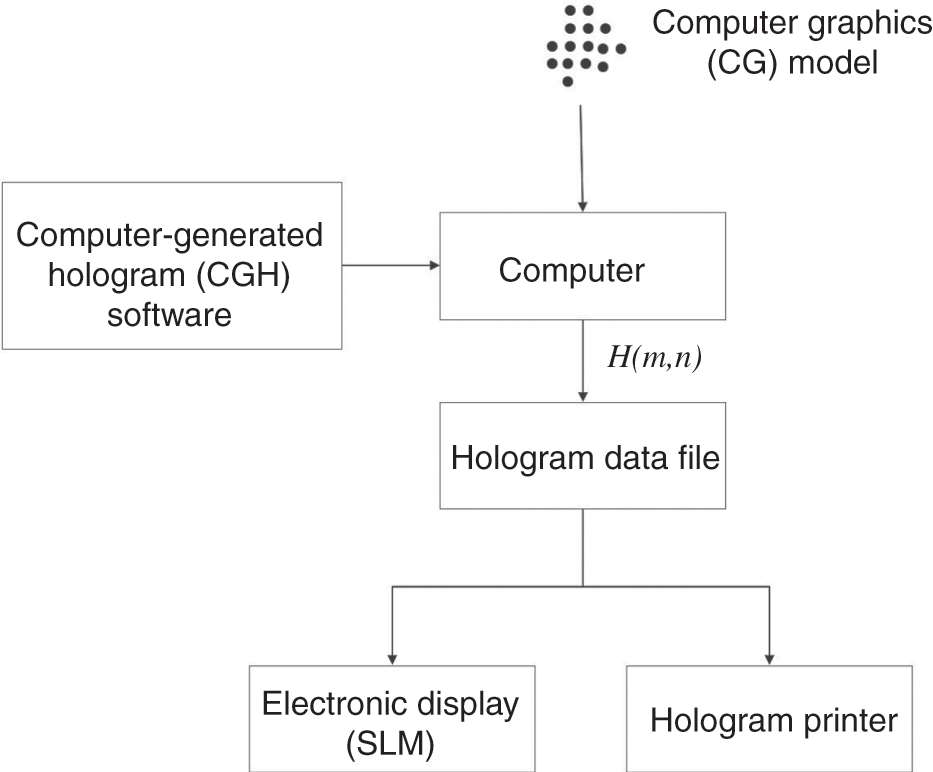
Figure 1.10 Computer-generated holography.
The set of self-illuminating points in the CG model is input into a computer, in which a software program is applied to compute a digital hologram of the CG model, and the result is stored in a data file. At this point, the data file is merely a set of numbers that does not provide a lot of clues about the object scene. As such, the data file is converted into a physical hologram by either printing it on a static medium (e.g., a photographic film) or displaying it on an electronic accessible device such as a spatial light modulator (SLM). An SLM is a device that is capable of spatially modulating the optical properties of light falling on or reflecting from it. Display chips such as liquid crystal (LC) and liquid crystal on silicon (LCoS) are typical examples of SLMs. In any case, the 3-D object scene will be reconstructed as a visible image that can be observed by our eyes when the hologram is illuminated with a coherent beam. The process of converting a 3-D CG model into a digital hologram is referred to as computer-generated holography.
The fundamental principles of CGH are introduced in this section. Euclidean space, terminologies, and parameters, which will be referenced throughout the book, are defined. Euclidean space, as shown in Figure 1.11, defines a 3-D virtual environment that houses the object scene and the hologram. There are two major parts in the environment: the object space and the hologram plane. The object space contains the 3-D object scene (i.e., the CG model) which is composed of one or more objects, while the hologram plane contains the digital hologram to be generated. Major parameters that are frequently used throughout the book are defined in Table 1.1, and outlined as follows. Locations in Euclidean space are addressed with discrete rectangular Cartesian coordinates, with m and n
and n (both of which are integers) denoting the discrete lateral (i.e., horizontal and vertical) coordinates. The axial direction, or the depth, that is orthogonal to the m
 and the n
 axes, is represented by the variable z. The hologram is assumed to be square in shape, with an identical number of rows and columns equal to H_DIM. The sampling intervals of the hologram and the lateral plane of the object space are identical and denoted by δd
 . Individual points in a hologram or an object scene are sometimes referred to as pixels. The physical location (x,y)
 of a discrete coordinate at (m,n)
 is related by (x,y)=(mδd,nδd)
 . The wavelength of light is denoted by λ
 .
.
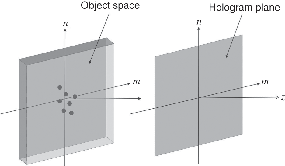
Figure 1.11 Spatial relation between the object space and the hologram plane.
Table 1.1 List of essential parameters
| Parameter | Symbol |
|---|---|
| Wavelength of light | λ |
| Sampling interval along the horizontal and vertical axes | δd |
| Horizontal extent of hologram and object space | H_DIM |
| Vertical extent of hologram and object space | H_DIM |
| Discrete horizontal coordinate | m |
| Discrete vertical coordinate | n |
| Axial coordinate (depth) | z |
Similar to optical holography, numerous research works have been conducted in CGH. There are two basic approaches in CGH, which are commonly known as the point-based method and the layer-based method. Both methods are straightforward and easy to implement, but the computation time is extremely lengthy. However, the latter part of this book will explain how this problem can be overcome with fast algorithms, leading to significant shortening of the computation time. As the point-based and layer-based methods are both important foundations of CGH, they will be described in more detail in the subsequent sections. In passing, there are other, more sophisticated techniques in CGH, such as polygon-based methods. However, they are beyond the scope of this book; interested readers may refer to [11–13] for details.
1.5.1 Point-Based Method
In the point-based method [14], the 3-D object scene is represented by a set of points Λ={o0,o1,…oP−1} , where P is the total number of object points. In some literature, where the object scene is presented as an image, object points are also referred to as pixels. Each object point in Λ
 is indexed by the variable p and characterized by its intensity Ap
 , its position (mp,np)
 on the lateral plane, and its axial distance zp
 from the hologram plane. The axial distance is often referred to as the depth of the object point. For a single point with unity intensity, and located at mp
 , np
, np , and depth = zp
 , its object wave impinging on the hologram can be obtained with Fresnel diffraction as given by
 (1.11)
 where rm;n;mp;np;zp=(m−mp, )2δd2+(n−np)2δd2+zp2 is the distance between an object point at (mp,np)
 on the image plane at depth = zp
 , to a pixel at (m,n)
 on the hologram.
If the object point is located at the origin (i.e., mp=np=0 ), the object wave is reduced to a more simple expression given by
 (1.12)
 a function that is commonly known as the Fresnel zone plate (FZP). If the separation between the object space and the hologram plane is sufficiently large (i.e., zp≫M;N ), the term rm;n;0;0;zp−1
 can be approximated as a constant term and discarded in the expression. In any case, it can be easily inferred from Eq. (1.12) that the function Op(m,n,mp,np;zp)
 is simply a translated version of the FZP, that is

If the object scene is represented by the set of points Λ , the object waves on the hologram plane can be computed as the superposition of the object waves of all the object points, each weighted by its intensity value Ap
 as
as
 (1.14)
 The function H(m,n) that records the collection of the object waves is known as a digital Fresnel hologram of the object scene, as it is obtained from the Fresnel diffraction equation in Eq. (1.11). Referring to the above formulation, the hologram is a complex-valued function. As the hologram is generated in a point-by-point manner, the process is generally known as the point-based method.
To illustrate the point-based method, a numerical simulation of generating a digital Fresnel hologram of a set of object points is demonstrated with the MATLAB codes in Section 1.8.1. In the simulation program the object space is derived from a source image comprising a pair of characters, “H” and “K,” having brightness of 255 and 128, as shown in Figure 1.12(a). Each non-zero pixel in the image is taken to be an object point. The image is evenly partitioned into a left half-plane, and a right half-plane that are located at 0.07 m and 0.08 m from the hologram, as illustrated in Figure 1.12(b). In another words, the object space is a double-depth image. The size of the hologram is 256 × 256. The optical settings, which will be adopted in all the simulation programs in this book, are shown in Tables 1.2.
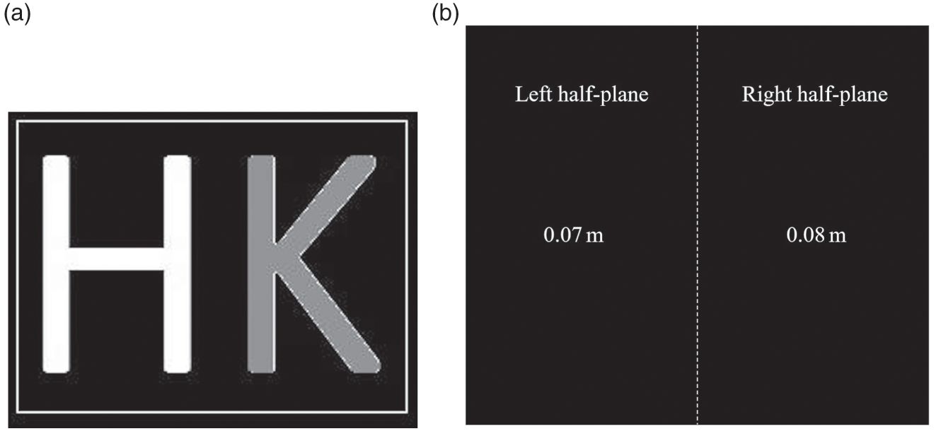
Table 1.2 Optical settings adopted in the simulation programs of this book
| Wavelength λ | 520 nm |
| Pixel size of hologram δd | 6.4 μm |
After running the main program, the Fresnel hologram is generated; the real and the imaginary parts of the hologram are displayed in Figure 1.13. It can be seen that the holographic images in both components are composed of high-frequency fringes that bear little resemblance to the original object image.
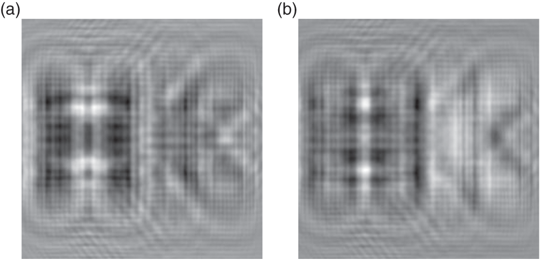
Figure 1.13 A digital Fresnel hologram of the double-depth image shown in Figure 1.12, generated with the point-based method and based on the optical settings in Table 1.2. (a) Real part of the hologram. (b) Imaginary part of the hologram.
1.5.2 Layer-Based Method
Although the point-based method is effective in generating the digital Fresnel hologram of a 3-D object scene, the computation will be extremely heavy if there are a lot of object points. For example, if the object space is a planar image of size 256×256 , there are over 64 000 object points, and the object wave of each of them has to be calculated and superimposed on the hologram. This problem can be alleviated with the layer-based method.
In the layer-based method, the 3-D object space is evenly partitioned into a sequence of D depth planes, denoted by ΓS=Ij(m,n)|1≤j≤D , which are parallel to the hologram as shown in Figure 1.14. Each depth plane is a 2-D image representing the intensity and spatial distribution of the object points that are residing on that plane, which are at the same depth zj
 from the hologram. If the intensity of the entire image is zero at a particular location on a depth plane, it means that no object point is there.
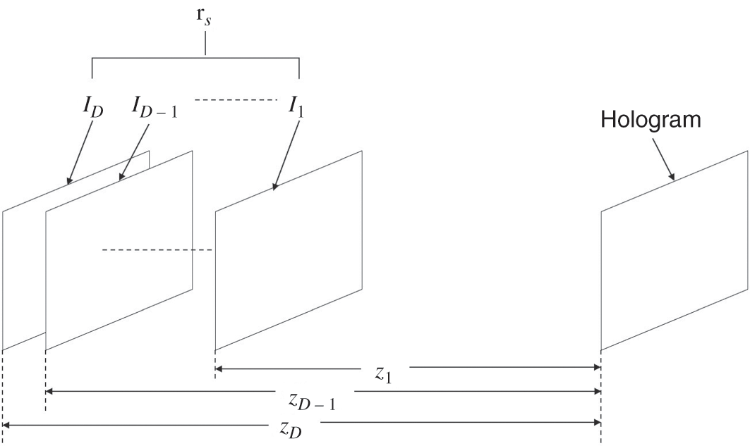
Figure 1.14 Partitioning the object space into a sequence of evenly spaced depth planes which are parallel to the hologram.
Applying the concept of the point-based method, the object wave of the object points on the jth depth plane is
 (1.15)
 Equation (1.15) can be rewritten as a convolution process as
 (1.16)
 The Fresnel hologram of the object scene is obtained from the sum of the object waves of all the depth planes, which can be expressed as
 (1.17)
 Replacing the arithmetic calculations in Eq. (1.15) with the convolution operation in Eq. (1.16) does not lead to any reduction in the amount of computation. However, to be described later, convolution can be speeded up significantly if it is implemented in the frequency instead of the spatial domain. In this respect, convolution has a definite advantage over the point-based method in generating a hologram. Besides, convolution can also lead to some convenience in software implementation. Apart from convolution, there are other improved techniques for applying the layer-based method, such as, among others, [15–17]. From Eq. (1.17) it can be inferred that the computation time will become more and more significant with increasing number of depth planes, as well as the size of the object space and the hologram. As such, the computation advantage of the convolution method is reduced in generating holograms of thick objects, in which case the depth range has to be partitioned into a large number of layers.
1.6 Reconstruction of Digital Hologram
The process of recovering a visual image of the 3-D object space from a hologram is known as reconstruction [18]. When a physical hologram (that is printed on a recording medium or displayed on an electronic accessible device) is illuminated with a coherent beam, a visible image of the 3-D object space can be observed from the hologram. This is generally referred to as optical reconstruction. For a digital hologram, reconstruction can be realized with computation, a process that is generally known as numerical reconstruction.
Hologram reconstruction can be interpreted as the reverse process of hologram generation, where the light beams are propagated from the hologram plane to the object space. This can be quite apparent in the case of an object scene with a single-depth plane at z=z1. Applying the layer-based method in Eq. (1.16), the Fresnel hologram H(m,n)
 corresponding to this single plane object is the convolution between the intensity image, and the FZP is
 (1.18)
 By inspection, the intensity image can be recovered from the hologram by convolving it with the conjugate of the FZP:
 (1.19)
 The same principle can be extended to the reconstruction of a hologram representing an object scene with multiple depth planes. Refer again to Eqs. (1.16) and (1.17) on a hologram that is generated with the convolution-based method. To reconstruct the image IR;k(m,n) located at the focused plane z=zk
 , Eq. (1.19) is applied to convolve the digital hologram with the complex conjugate of the FZP at the corresponding depth. Mathematically this is presented as
 (1.20)
 It can be seen that the image Ik(m,n) at the focused depth plane z=zk
 is fully recovered in the reconstructed image, while the rest of the depth planes are reconstructed as blurred, defocused content JR(m,n)
 . This is similar to how a 3-D scene is observed with eyes. When focusing on a near subject, those that are farther away will appear to be blurred, and vice versa.
As an example, a digital Fresnel hologram of the double-depth image in Figure 1.12 is generated with the layer-based method. From the generated hologram, the object scene, which is composed of two layers, is reconstructed from it in a plane-by-plane manner. The reconstructed images at the two depth planes are shown in Figures 1.15. In both cases, the character that is located at the focused plane is reconstructed as a sharp image, while the other is a blurred image. Apart from slight blurriness, the character that is reconstructed at its focused plane is similar to the original image. These results reflect the capability of a hologram in preserving the intensity and depth information of a 3-D object scene.

Figure 1.15 (a) Reconstructed image at depth plane 0.07 m. (b) Reconstructed image at depth plane 0.08 m.
1.7 Capturing Digital Hologram of a Physical Object
Although CGH can be employed to generate a hologram of a CG model, it cannot be applied directly – as in the case of optical holography – in capturing the digital hologram of a physical object. Referring to Figure 1.4, a digital hologram can be acquired by simply replacing the photographic film with a digital CCD camera. Similar to a photographic film, a CCD camera can only record intensity information. Hence, the off-axis hologram setup shown in Figure 1.6 is adopted in the capturing of a digital hologram. Since a digital camera comprises of a 2-D array of discrete optical sensors, the image recorded is also discretized in the same way. As such, the digital hologram H(x,y) will be replaced by its discrete form H(m,n)
 , where m
 and n
and n are integers representing the discrete coordinates along the horizontal and vertical directions. The following subsections introduce four methods for capturing digital holograms of a physical 3-D object.
1.7.1 Capture of Digital Off-Axis Hologram
Section 1.4 and Figure 1.7 infer that a digital off-axis hologram will suffer the same disadvantage as an optical off-axis hologram, with the virtual image being disrupted by the zero-order beam and the twin image. If the resolution of the digital hologram is not high enough, these three components will overlap each other, and a virtual image of the object space cannot be reconstructed correctly. Being different from a photographic film, which can have a very high resolution of less than 1 μm, the pixel size of a CCD camera is relatively much coarser. For example, the pixel size of a typical high-end scientific camera is around 5–7 μm. From the chart in Figure 1.9, the maximum angle of diffraction θmax is limited to the range [2.6∘,3.6∘]
 . Nevertheless, the off-axis arrangement is by far the most convenient way of acquiring a digital hologram.
Mathematically, the mechanism of capturing an off-axis hologram of a 3-D object scene is given by Eq. (1.7), and shown in the block diagram in Figure 1.16. A simulation of the process is provided in the MATLAB program given in Section 1.8.2.

Figure 1.16 Generation of digital off-axis hologram.
In the simulation, a digital Fresnel hologram of the double-depth image in Figure 1.12 is first generated with the layer-based method. After the hologram has been generated, a reference plane wave which is inclined at an angle of θR = 1.2° along the vertical direction is added to the hologram. The square of the magnitude of the mixed waves is taken to be the off-axis hologram, as shown in Figure 1.17(a). Next, the images at the two focused planes are reconstructed from the off-axis hologram, as shown in Figures 1.17(b) and 1.17(c). In each figure, it can be seen that the image of the character which is located at the focused plane is reconstructed clearly, while the other character becomes a defocused image. The bright square patch at the center is the zero-order beam, and the blurred region above it is twin image.

Figure 1.17 (a) Off-axis hologram of a double-depth image with θR = 1.2°. (b, c) Reconstructed image of the off-axis hologram at depth planes 0.07 m and 0.08 m, respectively.
A similar simulation is performed with the incidence angle θR being changed to 0.6°. The off-axis hologram is shown in Figure 1.18(a), and the reconstructed images at the two focused planes are shown in Figures 1.18(b) and 1.18(c). It can be seen that when the angle θR
 is small, the virtual image, twin image, and zero-order beam are overlapping and cannot be discriminated clearly.


1.7.2 Phase-Shifting Holography
It is desirable to capture both the amplitude and phase of the interference pattern of a hologram with a digital camera, so that the object scene can be fully reconstructed without being contaminated with the zero-order beam and the twin image. As mentioned previously, a digital camera can only record intensity information. This problem has been overcome with the phase-shifting holography (PSH) technique, which was first introduced in [19] for capturing electronic holographic signals with camera tubes.
In the basic PSH hologram acquisition method, an object specimen is illuminated by a coherent plane wave, which can be generated by expanding a laser beam with a beam expander. The object wave of the illuminated specimen (which is a complex-valued function) is sequentially added with four different phase-shifted versions of a reference wave that are derived from the illumination beam. The summation of the object wave with each version of the reference wave results in a beat, or interference pattern. The magnitude of each interference pattern, referred to as an interferogram, is captured by a camera. Subsequently, the complex-valued object wave of the specimen can be recovered from the four interferograms. Since four exposures are required to capture the interferograms, the method is known as four-step PSH.
The general optical setup of a PSH system is illustrated in Figure 1.19. A laser beam is expanded by the beam expander into a plane wave exp(iϕR) and split into two light beams by the beam splitter BS1. The first beam is reflected by the mirror M1, and directed to illuminate the specimen. The second beam propagates through a phase shifter (PS), whereby one of the four phase-shift values in the set PH4={0,π/2,π,3π/2}
 is added to form a phase-shifted reference plane wave exp(iϕR+iϕk)|ϕk∈PH
 . Next, the object wave O(m,n)
  emitted from the specimen is sequentially mixed with each of the reference beams, and the magnitude of the interference pattern (i.e., the interferogram) is recorded by the digital camera. Let |O(m,n)|
 and θ(m,n)
 denote the magnitude and phase of the object wave, respectively; the four interferograms are

 (1.21)
  (1.22)
  (1.23)
  (1.24)
 where C=(1+|O(m,n)|2) . It can be easily proved that
 (1.25)
 Apart from the additional constant phase term exp(iϕR) , which can be neglected in practice, the original complex object wave of the specimen is recovered.
A simulation of the four-step PSH hologram acquisition process in Figure 1.19 is conducted with the code listed in Section 1.8.3. The source image is the double-depth image shown in Figure 1.12, containing the characters H and K located at distances of z1=0.07 m and z2=0.08 m
 from the hologram. First, a hologram representing the double-depth image is generated with the layer-based method. Next, four interferograms are generated, each by adding the hologram with one of the four phase-shifted versions of the reference wave, and taking the magnitude of the result. For simplicity, the phase of the reference wave before passing through the phase shifter (PS) is assumed to be zero. After executing the program, the four intensity images of the interferograms captured by the CCD camera are shown in Figure 1.20(a–d). Next, the hologram is composed from the four interferograms, and the reconstructed images at the two focused planes are derived from the hologram and shown in Figures 1.20(e) and 1.20(f).

Figure 1.20 (a–d) The four interferograms corresponding to the hologram of the double-depth image in Figure 1.12. (e) Reconstructed image at depth plane 0.07 m. (f) Reconstructed image at depth plane 0.08 m.
Despite the effectiveness of the four-step PSH in capturing a complex-valued hologram of a physical 3-D object, the process is rather tedious as the four interferograms have to be captured. As each interferogram is formed by adding to the object wave a phase-shifted version of the reference wave, the capturing of the interferograms has to be conducted in a sequential manner. Over the years, quite a number of research investigations have been conducted to reduce the number of interferograms in a PSH system.
One of the early attempts to simplified the four-step PSH, known as the three-step PSH, was proposed by Y. Awatsuji et al. in [20]. In this approach, only three interferograms are captured, and these are integrated to recover the hologram of the 3-D object. The mechanism of the three-step PSH is similar to the four-step PSH, in which each interferogram is acquired by adding the object wave with one of the three phase-shifted versions, PH3={0,2π/3,−2π/3} , of the reference wave.
Mathematically, the three interferograms can be expressed as
 (1.26)
  (1.27)
  (1.28)
 It can be easily verified that
 (1.29)
 Subsequent to the three-step PSH, a two-step PSH [21–22] has been developed that only requires the acquisition of two interferograms, and the intensities of the object and the reference waves. Later, J.-P. Liu and T.-C. Poon [23] proposed a simplified method that does not require the recording of the reference and the object wave intensities.
Despite the improvements in PSH technology over the years, it requires the sequential acquisition of at least two interferograms, hence limiting its application to the imaging of stationary or very slow-moving specimens. In the case of recording a hologram of a fast-moving object, it is mandatory that all the interferograms are acquired concurrently. In [24], a parallel phase-shifting hologram (PPSH) method, as shown in Figure 1.21(a), is proposed. The reference wave is impinged on a phase-shifting array that contains downsampled version of different phase-shifting patterns. A small section of a typical phase-shifting array corresponding to a four-step PSH is shown in Figure 1.21(b). When the reference beam illuminates a particular cell in the phase-shifting array, it will be phase-shifted by one of the four values [0,π2,π,3π2] . The optical wave that emerges from the phase-shifting array comprises all the four phase-shifted version of the reference waves, which are spatially multiplexed in a non-overlapping manner. On the sensing plate of the camera, the object wave of the specimen mixes with a different phase-shifted version of the reference waves, resulting in four downsampled interferograms.

Subsequently each interferogram, after applying interpolation to fill in the missing pixels, is combined with Eq. (1.25) to obtain the hologram of the specimen. As all the interferograms are captured in a single round, the PPSH method is sometimes referred to as a parallel or one-step PSH.
By the same principle, the PPSH method can also be adopted to implement the three-step [20] and two-step PSH methods [21]. For each of these configurations, a phase-shifting array comprising triplets or pairs of phase-shifting pixels is overlaid onto the digital camera. With the PPSH, the interferograms are downsampled and need to be interpolated to their original size before being applied to compose the hologram. However, there are bound to be certain losses when the interferograms are downsampled, which cannot be fully recovered with interpolation. This will lead to distortion of the hologram composed from the interferograms, and hence its reconstructed image. The problem can be alleviated with a selective interpolation algorithm to include the sub-pixel data [25]. In comparison with linear interpolation, the selective interpolation method can lead to around 15% improvement of the reconstructed image of the hologram. Another interpolation method was proposed by Xia et al. [26], which is targeted at recovering the high-frequency signals in the downsampled interferograms. Later, the PPSH was applied in measuring the spectral reflectance of 3-D objects [27] and development of portable hologram-capturing systems [28,29].
The variants of the PSH methods have their pros and cons. Depending on the nature of the specimens and the precision required in capturing the holograms, different types of PSH methods may have to be used. For example, the single-step PSH is preferred for capturing the hologram of a dynamic object at the expense of introducing aliasing errors, while multiple-step PSH should be adopted for acquiring holograms with fewer errors. The above descriptions infer that switching between different PSH configurations will require changes in certain parts of the optical settings (e.g., replacing the phase-shifting array in changing a four-step PSH into a three-step PSH configuration). In view of this, a phase-mode SLM for generating the phase retardation patterns is proposed in [30].
1.7.3 Optical Scanning Holography
Sections 1.7.1 and 1.7.2 introduce two popular methods for recording holograms of physical objects. Both techniques are based on capturing, with a digital camera, the diffracted waves of the specimen that are illuminated with a coherent plane wave. A major disadvantage of these two methods is that the size and resolution of the hologram is limited by the receiving area of the image sensor. The coverage of the scene to be recorded, as well as the pixel size of the hologram, are therefore restricted by the image sensor.
The optical scanning holography (OSH) technique [31,32] developed by Poon and Korpel in the late 1970s, has overcome these restrictions. Based on a scanning mechanism and a single pixel sensor, the OSH is capable of capturing holograms of both microscopic and macroscopic objects. The full setup of an OSH system is rather complicated, and only a simplified concept is presented here. The hologram-capturing process of OSH can be divided into two stages. The first stage is shown in Figure 1.22(a), and explained as follows. The illumination beam Ψ(x,y;z) is a combination of a coherent plane wave and a coherent spherical wave that is generated from a point source, both having an optical frequency ω0
 . An acousto-optic modulator is used to modulate the frequency of the plane wave to (ω0+Ω)
 . For simplicity of description, the specimen is assumed to be a planar object that is parallel to the plane wave. Denoting the plane and the spherical waves by Aexp[i(ω0+Ω)t]
 , and Bexp[−ik02z(x2+y2)]exp[iω0t]
 , respectively, we have
 (1.30)
 where Ω is known as the heterodyne frequency and z
 is the axial distance between the specimen and the point source that generates the spherical wave.

Figure 1.22 First (a) and second (b) stages of optical scanning holography (OSH).
Utilizing an xy scanning device, the illumination beam is used to scan a specimen S along a zig-zag path. The optical waves scattered by the specimen are collected by a photo-detector through a focusing lens, resulting in a time-varying current i(x,y) . The zig-zag scanning of the specimen by the illumination beam can be described with a convolution process, as given by
 (1.31)
 After band-pass filtering with a filter tuned at the heterodyne frequency Ω , a signal iΩ(x,y)
 , which is known as the heterodyne current, results as
 (1.32)
 The second stage of an OSH system, which is used to extract the real and the imaginary components of the hologram of the specimen from the heterodyne current, is shown in Figure 1.22(b). The heterodyne signal iΩ(x,y) is input to a pair of mixers that multiply it with a cosine and a sine function. After mixing, the signals are low-pass filtered to give a signal ic(x,y)
 and a signal is(x,y)
 , as given by

and

where LPF[ ] denotes a low-pass filtering operation. The pair of signals ic(x,y) and is(x,y)
 , which are referred to as the cosine and the sine hologram, are the real and the imaginary components of the hologram of the specimen, respectively.
1.7.4 Non-diffractive Optical Scanning Holography
The optical and electronic setups in a classical OSH, as described in Section 1.7.3, are rather complicated. The scanning beam is composed of a spherical wave and a plane wave that is modulated with a low-frequency sinusoidal wave at the heterodyne frequency. As the pair of beams have to be integrated into a single scanning beam, all the elements in the optical setups have to be positioned and aligned precisely. Subsequently, a pair of mixers are used to extract the cosine and sine holograms from the heterodyne signal of the photo-detector. Non-diffractive optical scanning holography (ND-OSH) [33,34] is a simplified version of OSH that can be realized with very few optical and electronics accessories. The ND-OSH system is shown in Figure 1.23. In ND-OSH, a pair of image patterns, gR(m,n;z) and gI(m,n;z)
 , are projected from a commodity projector. The two image patterns are given by

Figure 1.23 Non-diffractive optical scanning holography (ND-OSH) system.
 (1.34a)
 and
 (1.34b)
 The specimen is sequentially scanned by the pair of image patterns along a zig-zag path, and a single pixel sensor is employed to record the reflected light. Scanning can be conducted by mounting the specimen on an X–Y platform that moves along a row-by-row and left-to-right path. The output signals of the single pixel sensor are two intensity images (each corresponding to one of the image patterns) representing the convolution between the 3-D image of the specimen and the pair of image patterns. Suppose the specimen is represented by a stack of D image planes Ij(m,n)|1≤j≤D , each located at depth zj
 (see Figure 1.14). Scanning of each depth plane results in two signals:
 (1.35a)
 and
 (1.35b)
 In Eqs. (1.35a) and (1.35b), hR(m,n;zj) and hI(m,n;zj)
 can be identified as the real and imaginary components of the hologram of the image plane Ij(m,n)
 , added with a constant term C. The hologram of the entire specimen can be obtained from these two components, as given by

where C′=D×C is the overall intensity of the specimen, which can be obtained by exposing the specimen to a uniform white light and measuring the output of the photo-detector. Similar to classical OSH, ND-OSH does not place rigid constraints on the coverage of the object scene and the size of the hologram.
1.8 MATLAB Simulation
This section includes the MATLAB source codes that are employed to conduct the simulations of the methods reported in this chapter. A summary of the simulation programs (each identified by the name of its main function call) and their correspondence to sections in the chapter are listed in Table 1.3.
Table 1.3 Summary of simulation programs in Chapter 1
| Function name | Description of simulation | Associated sections |
|---|---|---|
| Point_based | Computer-generated hologram of a double-depth image with the point-based method | 1.5.1 |
| Off_axis | Simulation on capturing an off-axis hologram of a double-depth image | 1.7.1 |
| PSH | Simulation on capturing a hologram with the phase-shifting holography method | 1.7.2 |
The image “HK1” with the intensity distribution and depth map shown in Figures 1.12(a) and 1.12(b), respectively, is adopted in the simulation programs. The image is evenly divided into a left half-plane and a right half-plane, containing the characters H and K, respectively. The left half-plane is located at a distance of 0.07 m from the hologram plane, while the right half-plane is placed farther away at 0.08 m.
1.8.1 Simulation of Generating a Hologram with the Point-Based Method
The MATLAB code for this simulation is shown in Table 1.4. A digital Fresnel hologram of the double-depth image in Figure 1.12 is generated with the point-based method. The main function “Point_based” is called to load the source image file. Next, the function “PB_hologram” is called. Each object point is extracted from the source image and its diffraction pattern, which is in the form of an FZP, is added to the hologram. Upon completion of the process, a digital Fresnel hologram of the double-depth image is generated. Subsequently, the hologram and its reconstructed images on the two focused planes are displayed and saved.
Table 1.4 MATLAB code of the point-based method for generating a digital Fresnel hologram of a set of object points
1.8.2 Simulation of Capturing an Off-Axis Hologram
This simulation, with the MATLAB code shown in Table 1.5, demonstrates capture of an off-axis hologram of a double-depth image. The main function “Off_axis_holo” is called to load the double image in Figure 1.12, and converts it into a digital Fresnel hologram with the function “Holo_gen.” Next, the function “Off_Axis” is called to generate a plane wave that is inclined at an angle specified by the user. The inclined plane wave is added to the hologram, and the square of the magnitude of the hologram is taken to be the off-axis hologram. Subsequently, the reconstructed images at the two focused planes are computed, displayed, and saved.
1.8.3 Simulation of Capturing a Digital Fresnel Hologram with Four-Step Phase-Shifting Holography
Table 1.6 shows the MATLAB code for simulating the capture of a digital Fresnel hologram with four-step PSH. The main function “PSH,” is called to load the double-depth image shown in Figure 1.12. The function “Holo_gen” is called to generate a complex-valued hologram of the double-depth image. Four interferograms are generated by mixing each hologram with one of the four phase-shifted versions of the reference plane wave. The four interferograms are then combined into a digital Fresnel hologram. Subsequently the reconstructed images at the two focused planes are computed, displayed, and saved.
1.9 Summary
In Sections 1.1–1.4, the fundamental principles of optical holography for capturing the optical waves of physical objects, and its difference from photography, are described. An image taken with photography, commonly referred to as a photograph, can only record a single view of an object scene. A hologram is capable of capturing the entire optical wavefront that impinged on it. As such, there should be little difference between observing a hologram and the physical object scene.
Numerical generation of a digital hologram, a technology that is commonly known as computer-generated holography, is presented in Section 1.5. Two important approaches in CGH – the point-based and the layer-based methods – are described. From the computational efficiency point of view, the point-based method is suitable for generating holograms of simple objects that comprise a small number of object points. However, for an object scene with large number of object points concentrated in a few depth planes, the layer-based method is preferred. The method for recovering a 3-D scene image from a digital hologram is provided in Section 1.6.
| function PSH() | |
| close all | |
| clc | |
| warning off | |
| fname=‘HK1‘; | |
| I=imread(strcat(fname,’.jpg’)); | %Filename of intensity image |
| I=im2double(I); | |
| [N M]=size(I(:,:)); | %Size of source image identical to size %of hologram |
| I1=I; | %First layer |
| I1(:,M/2+1:M)=0; | %Only left half-plane of source image in %first layer |
| I2=I; | %Second layer |
| I2(:,1:M/2)=0; | %Only right half-plane of source image %in second layer |
| psize=6.4*10^-6; | %Pixel size of hologram=6.4 μm |
| lamda=540*10^-9; | %Wavelength=540 nm |
| %Generate object wave of image on first depth plane with the correlation-based %method | |
| z1=0.07; | |
| H=Holo_gen(I1,z1,psize,lamda); | |
| %Generate object wave of image on second depth plane with the correlation-%based method | |
| z2=0.08; | |
| H=H+Holo_gen(I2,z2,psize,lamda); | |
| MAX=max(abs(H(:))); | |
| H=H/MAX; | |
| IN1=abs(H+exp(1i*0)).^2; | |
| IN2=abs(H+exp(1i*pi/2)).^2; | |
| IN3=abs(H+exp(1i*pi)).^2; | |
| IN4=abs(H+exp(1i*3*pi/2)).^2; | |
| figure,imshow(mat2gray(IN1)); | %Display interferogram 1 |
| title(‘1st interferogram’); | |
| figure,imshow(mat2gray(IN2)); | %Display interferogram 2 |
| title(‘2nd interferogram’); | |
| figure,imshow(mat2gray(IN3)); | %Display interferogram 3 |
| title(‘3rd interferogram’); | |
| figure,imshow(mat2gray(IN4)); | %Display interferogram 4 |
| title(‘4th interferogram’); | |
| imwrite(mat2gray(IN1),’Holo_PSH_1.jpg’); | |
| imwrite(mat2gray(IN2),’Holo_PSH_2.jpg’); | |
| imwrite(mat2gray(IN3),’Holo_PSH_3.jpg’); | |
| imwrite(mat2gray(IN4),’Holo_PSH_4.jpg’); | |
| %Compute real and imaginary components of the hologram from the four %interferograms | |
| HR=(IN1-IN3)/4; | |
| HI=(IN2-IN4)/4; | |
| %PSH hologram | |
| G=(HR+1i*HI); | |
| %Reconstruct images at the two focused planes from the PSH hologram | |
| RES1=abs(Holo_recon(G,z1,psize,lamda)); | |
| figure,imshow(mat2gray(RES1)); | |
| title(‘Reconstructed image of PSH hologram at depth = z1’); | |
| RES2=abs(Holo_recon(G,z2,psize,lamda)); | |
| figure,imshow(mat2gray(RES2)); | |
| title(‘Reconstructed image of PSH hologram at depth = z2’); | |
| imwrite(mat2gray(RES1),’RES_PSH_D1.jpg’); | |
| imwrite(mat2gray(RES2),’RES_PSH_D2.jpg’); | |
| end | |
| function H=Holo_gen(I,z,psize,lamda) | |
| [N M]=size(I(:,:)); | |
| wn=2*pi/lamda; | %Wave number |
| H=zeros(N,M); | |
| %Generate Fresnel zone plate | |
| z2=z*z; | %Square of the depth value z |
| [kx ky]=meshgrid(-M/2:M/2–1,-N/2:N/2–1); | |
| kx=kx*psize; | %Physical horizontal position |
| ky=ky*psize; | %Physical vertical position |
| fzp=exp(1i*wn*sqrt(kx.^2+ky.^2+z2)); | |
| %Generate hologram | |
| H0=conv2(fzp,I); | |
| [N0 M0]=size(H0(:,:)); | |
| %Crop the hologram to its original size H_DIM | |
| H=H0((N0-N)/2:(N0+N)/2–1,(M0-M)/2:(M0+M)/2–1); | |
| end | |
| function RES=Holo_recon(H,z,psize,lamda) | |
| [N M]=size(H(:,:)); | %Size of input hologram |
| wn=2*pi/lamda; | %Wave number |
| %Generate Fresnel zone plate | |
| z2=z*z; | %Square of the depth value z |
| [kx ky]=meshgrid(-M/2:M/2–1,-N/2:N/2–1); | |
| kx=kx*psize; | %Physical horizontal position |
| ky=ky*psize; | %Physical vertical position |
| r=sqrt(kx.^2+ky.^2+z2); | |
| fzp_c=exp(-1i*wn*r)./r; | %Conjugate of FZP |
| IR=conv2(H,fzp_c); | |
| [NR MR]=size(IR(:,:)); | |
| %Crop to include only the region containing the reconstructed image | |
| RES=IR((NR-N)/2:(NR+N)/2–1,(MR-M)/2:(MR+M)/2–1); | |
| end | |
Approaching the end of this chapter, in Section 1.7 three different methods for capturing digital holograms of the physical object scene are described. The first method is similar to the art of optical holography, but instead of a photographic film, a digital camera is used to record the holographic waves emitted from the scene. As a digital camera can only record intensity information, the method can only be employed to capture an off-axis, amplitude-only hologram. The other two methods, known as phase-shifting holography and optical scanning holography, are capable of capturing both the magnitude and phase components of the holographic signals. The PSH is faster in operation, while the OSH can be used to capture holograms of large objects. Finally, a simplified version of OSH, known as non-diffractive optical scanning holography, is presented. ND-OSH is similar in principles to OSH, but the complexity of the optical and electronic setups is reduced.
Exercises
E.1.1 Referring to Figures 1.5(a) and 1.5(b), a pinhole camera is used to cast the image of two points, A and B, onto an image plane that is located at an axial distance of 0.03 m from the pinhole. The horizontal and vertical coordinates (in meters) of A, B and the pinhole are (0.01, 0.0), (0.005, −0.003), and (0.0, 0.0), respectively. Determine the positions of A′, B′ on the image plane.
E.1.2 The expression of a Fresnel zone plate (FZP) is given in Eq. (1.12). Given λ=0.52 μm
 , δd=6.4 μm
 , and H_DIM = 2048, write a MATLAB program to display the magnitude and phase components of an FZP at different values of zp
 , and explain why the distance zp
 has to be sufficiently large in the generation of a digital Fresnel hologram.
E.1.3 Based on the optical settings in the previous question, perform a simulation with MATLAB to compare the computation time between generating a hologram of the single-depth image in Figure 1.12 with (a) the point-based method, and (b) the layer-based method. Repeat the above simulation with images comprising fewer object points. From the results, evaluate the pros and cons of these two methods in the generation of digital Fresnel holograms.
E.1.4 Extend the MATLAB codes in Section 1.8.2 to generate off-axis holograms of the double-depth image in Figure 1.12, based on a reference wave that is (a) inclined at an angle of 1.2° along the horizontal direction, and (b) inclined at an angle of 1.2° along both the horizontal and the vertical directions.
E.1.5 Modify the MATLAB codes in Section 1.8.3 to conduct a simulation of the four-step parallel phase-shifting holography method based on the phase-shifting array in Figure 1.21(b) for acquiring a digital Fresnel hologram of the double-depth image in Figure 1.12.
E.1.6 Perform a literature study on references [20] and [21]. Subsequently conduct a MATLAB simulation on the three-step and the two-step parallel phase-shifting holography method for acquiring a digital Fresnel hologram of the double-depth image in Figure 1.12.


