Abstract
Phase-only Fresnel holograms have two major advantages over complex-valued or amplitude-only hologram. First, they can be displayed with a single phase-only SLM, leading to simplification on the holographic display system. Second, due to the high optical efficiency of phase-only holograms, the reconstructed image is brighter than that of an amplitude-only hologram. On the downside, the fidelity of the reconstructed image is degraded as a result of discarding the magnitude component of the hologram. In this chapter, a number of methods, each with pros and cons, for generating phase-only holograms are described. These methods can be divided into two types, iterative and the non-iterative. Iterative methods include the iterative Fresnel transform algorithm (IFTA) and its variants, which find their origin in the classical Gerchberg–Saxton algorithm (GSA). Reconstructed images of a phase-only hologram obtained with IFTA are generally good in quality, but the computation time is rather lengthy. Another iterative method, based on direct binary search (DBS), can be applied in generating binary phase-only holograms. Non-iterative methods are based on modifying the source image in certain ways prior to the generation of the hologram. These include noise addition, patterned phase addition, and downsampling. The modification is similar to overlaying a diffuser onto the image, so that the magnitude of the diffracted waves on the hologram is close to homogeneous. The phase component alone, therefore, can be taken to represent the hologram.
3.1 General View on Holographic Display System
Some of the important methods that are employed in the generation of digital Fresnel holograms have been introduced in the previous chapters. As mentioned before, a digital hologram is merely an array of complex-valued data, which is not meaningful to the real world unless it can be converted into a physical hologram and used to display a visible holographic 3-D image. An early approach to forming a physical hologram from digital holographic data was to generate a real off-axis hologram (see Sections 1.4 and 1.7.1) and to print it with a high-resolution printer. Printer technology has advanced significantly in the past two decades; it is now possible to hardcopy holograms with resolution of over 2400 dots-per-inch (dpi) through a commodity laser printer. Even higher printing resolution can be achieved with professional image setters or holographic fringe printers. In general, the higher the resolution of the printing device, the better will be the quality of the reconstructed image of a hologram. Despite these encouraging developments in hologram printing, the content of a printed hologram is not refreshable and can only record a static scene.
The advancement of electronic display technology has provided the green light to the display of dynamic holographic images. At the time of writing, display devices such as liquid-crystal-on-silicon (LCoS), with a pixel size of around 3 μm are available at an affordable price. Although the size of these devices is generally small, they are sufficient for showing a medium-size hologram with good visual quality. In the study of holography, high-resolution electronic displays are generally referred to as spatial light modulators (SLMs), meaning that the optical properties of light (such as polarization, phase, and amplitude) could be changed when the optical beam is transmitted or reflected from the device. However, SLMs developed to date are only capable of changing either the amplitude or the phase component of an optical signal. An SLM that is configured to modulate the amplitude or phase component is referred to as an amplitude-only SLM or a phase-only SLM, respectively. In either configuration, a single SLM is inadequate for displaying a hologram comprising complex-valued pixels.
3.1.1 Dual SLM Holographic Display System
To overcome this problem, a holographic display formed by the cascade of a pair of SLMs is proposed by C. Stolz et al. [1] and R. Tudela et al. [2]. The optical setup is shown in Figure 3.1. The first SLM modulates the amplitude of the illumination beam according to the amplitude component of the hologram, while the second SLM modulates the phase of the optical wave according to the phase component of the hologram. The light wave that emerges from the two SLMs will be equivalent to the holographic signal emitted from the hologram, from which a reconstructed image of the 3-D scene can be observed. Although this is a straightforward implementation, the setup is bulky and expensive as two SLMs are involved. Due to the fine resolution of the display devices, precise optical alignment is required to ensure the correct amplitude and phase modulation of every light beam that passes through every pair of corresponding pixels of the two SLMs. Nevertheless, the method is effective and further research works have been conducted along this direction. An alternative two-SLM approach has been reported by L. Zhu and J. Wang [3] and A. Siemion et al. [4], who decomposed a complex-valued hologram into a pair of phase components, and displayed them with two cascaded phase-only SLMs. The concept has been extended by M. Makowski and his co-workers for displaying color Fourier holograms [5].
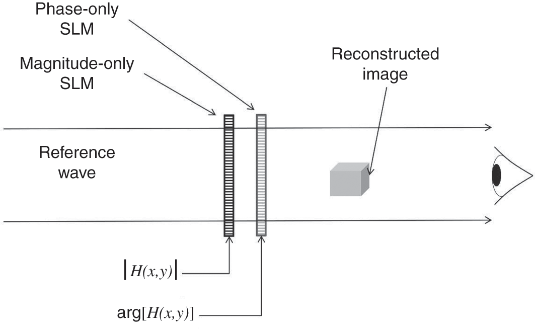
Figure 3.1 Concept of a dual, magnitude–phase coupled SLM holographic display system.
3.1.2 Split SLM Holographic Display System
The optical setup in Figure 3.1 can be much simplified if only a single SLM is used in the display system. Such an attempt has been made by Liu et al. [6] with the setup shown in Figure 3.2. Instead of separating the real and the imaginary components into two different SLMs, they are multiplexed on a single SLM. Referring to Figure 3.2, an amplitude-only SLM is uniformly split into two areas. The real component HR(m,n)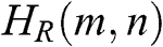 and the imaginary component HI(m,n)
 of a complex-valued hologram are each displayed on one of these two areas. When the SLM is illuminated with a coherent wave, the optical beam that passes through each section is amplitude-modulated by the hologram pixels on it. The modulated light waves from the two sections are then merged to form the holographic signal of the hologram through some optical devices. From the holographic signal, a visible 3-D image of the object scene that is represented by the original complex hologram will be reconstructed.
Figure 3.2 A partitioned, single SLM holographic display system.
A different solution, which is also based on the split SLM configuration, has been proposed by H. Song et al. [7]. A hologram is decomposed into a pair of phase components, with each of them being displayed in separate sections on a phase-only SLM. Similar to [6], the SLM is illuminated with a coherent beam, and the optical waves emitted from the two sections are merged optically to give the complex-valued holographic signal.
There are two major problems associated with the split SLM display system. First, as a single SLM is used to display the two components of a complex-valued hologram, the display area is reduced by two times. The size of the hologram, and hence the space–bandwidth product, are decreased by the same factor. As a result, the field of vision of a hologram displayed on a split SLM is smaller than that of a single SLM. Second, optical accessories such as lenses and high-resolution gratings are required to combine the optical wave from the two sections of the SLM. The alignment of the SLM and the optical accessories has to be very precise. Otherwise, the two components of the hologram cannot be integrated to recover the original holographic signal and are heavily distorted on the reconstructed image. In view of these issues, it is desirable if a hologram can be encapsulated into a single component (either the amplitude or the phase component), so that it can be displayed with a single, non-partitioned SLM.
3.1.3 Amplitude-Only SLM Holographic Display System
In the study of optical holography in Section 1.4, a hologram can be represented solely by its magnitude component if it is mixed with an inclined reference wave. This is the classic way of recording hologram onto a photographic film. Following the same principle, an amplitude-only SLM can be used to display an off-axis hologram as the values of all the pixels are real quantities. As explained in Section 1.4, there are two major drawbacks. First, the reconstructed image of an off-axis hologram is accompanied by the zero-order beam and the twin image, both of which may contaminate the virtual image if the pixel size of the SLM is not fine enough. Second, the optical efficiency of an amplitude-only hologram is rather low, as hologram pixels are translucent (i.e., having transmissivity between opaque and transparent), which blocks or fails to reflect some of the light energy.
A second solution is to display the phase component of a hologram alone by modulating the phase angle of the optical beam that impinges on it. Being different from an amplitude-only hologram, the optical efficiency of a phase-only hologram is high, as the transmissivity of hologram pixels is close to 100%, and only the phase angle of the optical beam is changed. However, direct removal of the magnitude component of a hologram will lead to heavy distortion in the reconstructed image. To overcome this problem, the hologram has to be generated in a way that the magnitude component is more or less homogeneous. Such kind of holograms are referred to as phase-only holograms. In the past few decades there have been numerous research efforts to explore methods for generating phase-only holograms. In the subsequent part of this chapter, different methods that have been developed in recent years on the generation of phase-only Fresnel hologram will be reviewed.
3.2 Iterative Method for Generating Phase-Only Holograms
3.2.1 Generating Phase-Only Hologram for a Single-Depth Image
The Gerchberg–Saxton algorithm, often referred to as GSA [8], is by far one of the most popular approaches for generating a digital phase-only hologram. The algorithm, named after its two inventors, Gerchberg and Saxton, was originally used to retrieve the phase of a pair of related light distributions. The principles of GSA have been extended to the generation of digital phase-only Fourier holograms. A Fourier hologram is a complex-valued image that is obtained from the Fourier transform of an image. Similar to what was mentioned in Section 3.1, it will be desirable to convert it into a phase-only component to increase the optical efficiency.
Figure 3.3 depicts a variation of the GSA known as the “iterative Fourier transform algorithm” (IFTA), which is applied to generate a phase-only Fourier hologram. The pair of light distributions are the intensity I(m,n) of the source object on the image plane and its digital Fourier hologram H(m,n)
 on the hologram plane. The objective is to derive a hologram so that the reconstructed image of its phase component HP(m,n)
 is similar to I(m,n)
 . Intuitively, this seems to contradict the theory of holography as the phase component of a hologram alone is insufficient to recover the original image. However, this dilemma can be alleviated if HP(m,n)
 is being solely required to reconstruct a modified version of I(m,n)
 given by J(m,n)≈I(m,n)eiϕ(m,n)
 , where eiϕ(m,n)
 is a pure phase term. The latter provides an extra dimension of freedom for partially absorbing the distortion caused by dropping the magnitude component of the hologram. As human perception only responds to the intensity of light, introduction of the extra phase term does not affect the appearance of the image. In IFTA, computation of a phase-only hologram HP(m,n)
 is obtained through repetitive rounds of iterations, explained below.

To start with, let t denote the current round of iteration, and Gt(m,n)=eiϕt(m,n) is the phase-only hologram obtained in the current epoch. Initially, at t=0
 , each pixel in the phase-only hologram ϕt=0(m,n)
 is assigned a random value within the range [−π,π]
 .
.
Next, the phase-only hologram is inverse Fourier transformed to a complex image Jt(m,n)=|Jt(m,n)|eiθt(m,n) on the image plane, as given by
 (3.1)
(3.1) Subsequently, an amplitude constraint is imposed with which the magnitude of Jt(m,n) is replaced by I(m,n)
 , resulting in a phase-added image IPt(m,n)=I(m,n)eiϕt(m,n)
 . The phase-added image IPt(m,n)
 is then Fourier transformed into a Fourier hologram Ht(m,n)=|Ht(m,n)|eiϕH;t(m,n)
 :
:
 (3.2)
(3.2) and the phase component ϕH;t(m,n) of the hologram is retained as the phase-only hologram Gt+1(m,n)
 , completing the current round of iteration. The conversion of the signals from the image plane to the hologram plane, and vice versa, is commonly referred to as forward and backward propagation, respectively.
The above process is repeated for a certain number of epochs, or until the difference between I(m,n) and |Jt(m,n)|
 is below a preset threshold. Note that in Eq. (3.2), the amplitude constraint is imposed so that the magnitude of the image to be converted to the hologram is always enforced to be identical to the original image I(m,n)
 . The phase term eiϕt(m,n)
 is allowed to vary freely according to the recent round of iteration. This has the effect of absorbing part of the errors caused by retaining only the phase component of the hologram. Upon completion of the process at the Tth epoch, the phase component GT(m,n)=eiϕT(m,n)
 is taken to be the phase-only hologram HP(m,n)
 . With more iterations, the reconstructed image of HP(m,n)
 will become increasingly similar to the source image I(m,n)
 .
.
The IFTA for generating Fourier phase-only holograms can be easily extended to the generation of Fresnel phase-only holograms, simply by replacing the forward/inverse Fourier transform with the forward/inverse Fresnel transform in Figure 3.3. This IFTA approach reported in [9].
There are several major disadvantages of the IFTA. First, for an arbitrary source image it is almost impossible to estimate how many rounds of iterations are required to generate the desired phase-only hologram (i.e., one with a reconstructed image that is close to the original one). Second, the reconstructed image is quite noisy as a result of the distortions caused by removing the magnitude component of the hologram. Third, the errors that can be absorbed into the phase term eiϕT(m,n) are quite limited. As a result, it is unlikely that the quality of the reconstructed image of HP(m,n)
 can be improved significantly simply by increasing the number of iterations. Fourth, as shown in Figure 3.3, the IFTA is only applicable for generating the phase-only hologram of a planar image that is parallel to the hologram plane. The subsequent parts of this section will demonstrate a number of methods for improving the performance of IFTA.
Simulation of the IFTA for generating the Fresnel hologram of a single-depth image is illustrated with the MATLAB code shown in Section 3.4.1. The object space adopted in the simulation is the single-depth image “Apple,” shown in Figure 3.4(a), which is located at an axial distance of 0.08 m from the hologram. The image is converted into a phase-only Fresnel hologram with the IFTA method. The reconstructed images on the focused plane of the phase-only holograms that are generated with one, three, and five iterations of the IFTA are shown in Figure 3.4(b–d). In the reconstructed images, only the region that is occupied by the image of the apple is shown. The reconstructed images are similar to the source image, and contaminated with a certain amount of random noise. With more iterations, the noise level is lowered and the reconstructed images become clearer.

Figure 3.4 (a) Source image “Apple.” (b–d) Reconstructed image from a phase-only Fresnel hologram that is generated with one, three, and five round(s) of IFTA, respectively.
3.2.2 Enhanced IFTA: Mixed-Region Amplitude Freedom Method
In Section 3.2.1, the reconstructed image of a phase-only hologram generated with the IFTA suffers noise contamination and slight distortion. The noise signal is caused by the removal of the magnitude component in the hologram, and although part of it can be absorbed into the phase term eiϕT(m,n) through the IFTA, the remaining ones will be distributed rather uniformly as random noise in the reconstructed image. In other words, every part of the reconstructed image will be added with a certain amount of random noise. After a certain number of iterations, there will not be further improvement of the noisy appearance of the reconstructed image. To overcome this problem, an enhanced IFTA method known as “mixed-region amplitude freedom” (MRAF) was proposed in [10]. The method was intended for designing holographic atom traps, but it can also be applied in generating phase-only Fourier or Fresnel holograms. In essence, the source image of the object is housed inside a new image of a larger size, so that the majority of noise resulting from the IFTA can be dispatched to the region that is not occupied by the source image. Details of the MRAF method are shown in Figure 3.5.

Figure 3.5 The “mixed-region amplitude freedom” (MRAF) for generating a phase-only Fresnel hologram, with the incorporation of the signal and the noise regions.
The source image I(m,n) is first moved to the center of a larger canvas, resulting in a bigger image IE(m,n)
 . The part that is occupied by I(m,n)
 (i.e., the dotted region) and the remaining areas on IE(m,n)
 are labeled as the “signal region” S and the “noise region,” respectively. Initially, at time t=0
 , the pixels of the phase-only hologram GE;t=0(m,n)
 are assigned random values within the range [−π,π].
Next, the phase-only hologram is inverse transformed to the reconstructed image JE;t(m,n)=|JE;t(m,n)|eiϕt(m,n) . On the image plane, the image IPE;t(m,n)
 is obtained by applying an amplitude constraint on JE;t(m,n)
 :
:
 (3.3)
(3.3) Equation (3.3) shows that the amplitude constraint enforces the signal region of the reconstructed image to duplicate the source image, whereas in the area covered by the noise region the reconstructed image is not altered. Grossly speaking, the noise region is not subject to amplitude constraint and can be altered freely in the iterative process. As the noise region is separated from the signal region containing the source image, it can be used to accommodate part of the distortions that are caused by removing the magnitude component of the hologram.
The amplitude constraint image is then forward transform to its hologram, and the phase component is retained as the phase-only hologram GE;t(m,n) , completing the current round of iteration. The above process is repeated until certain criteria, such as reaching the maximum number of iterations, have been met. In each round of iteration, the image within the signal region S is preserved, while the signal in the noise region will be altered, progressively shifting the noise signal from the signal region to the noise region.
Simulation of the MRAF with the incorporation of the signal and noise regions is conducted with the program given in Section 3.4.2. The reconstructed images of the phase-only holograms that are generated with one, three, and five iterations of the MRAF method are shown in Figure 3.6(a–c). The reconstructed image is composed of the image of the apple in the signal region, together with a noisy background in the noise region. Magnified views of the images in the signal region are shown in Figure 3.6(e–g), and for comparison the original image “Apple” is shown again in Figure 3.6(d). Compared with the results in Figure 3.4(b–d), it is evident that the noise contamination on the reconstructed images has been reduced.

3.2.3 Noise Reduction with IFTA Multiple Frame Averaging
The quality of a phase-only hologram HP(m,n) generated with IFTA is dependent on the initial randomization of the phase values of the hologram pixels. Suppose the object space is a single planar image I(m,n)
 that is parallel to the hologram plane, the reconstructed image I(m,n)
 of the phase-only hologram can be expressed as
 (3.4)
(3.4) where ℵ represents the noise contamination of the reconstructed image, which is dependent on the initial condition.
To reduce the noise contamination, IFTA is applied to generate a set of phase-only holograms of the same input image, each initialized with different phase randomization. Each of the holograms is referred to as a sub-hologram. Due to the deviation in initial conditions, the reconstructed images of each sub-hologram will be added with a different noise signal. The expectation of the reconstructed image J(m,n) obtained from averaging the reconstructed images of all the sub-holograms is given by

If the initial randomization is based on white noise, it is likely that the noise in the result will also be similar to white noise. With a sufficient number of samples, E[ℵ] will be close to a homogeneous background and E[J(m,n)]
 is practically equivalent to the source image.
The above principle can be applied to reduce the noise signal in an IFTA-generated phase-only hologram, and is outlined as follows. To start with, a set of phase-only sub-holograms representing the same source image is generated with the IFTA based on different initial randomization. Subsequently, the sub-holograms are displayed in rapid succession on an SLM. Due to the persistence of vision of human perception, the sequence of reconstructed images will appear to be merged into a single image. If the number of sub-holograms is sufficiently large, the reconstructed image will be close to the source image.
Simulation of this IFTA multiple frame averaging (IFTA-MFA) noise reduction method is conducted here. Similar to previous simulations, the object space is the single-depth image “Apple” in Figure 3.4(a). In the simulation, two or more phase-only sub-holograms are generated with the IFTA under different initial randomizations of the holograms. The magnitude of the reconstructed images of these sub-holograms on the focused plane are averaged to simulate the persistence-of-vision effect.
The reconstructed images obtained with the averaging of 2–5 frames of phase-only sub-holograms that are generated with one iteration of IFTA are shown in Figures 3.7(a–d). Compared with the results in Figure 3.4, it is evident that the noise contamination of the reconstructed images has been reduced, even though only one iteration has been applied in the generation of each phase-only sub-hologram.

Figure 3.7 Averaging multiple frames of reconstructed images of phase-only Fresnel holograms that are generated with one iteration of IFTA, but under different initial random noise (a)–(d) averaging 2–5 frames, respectively.
The IFTA-MFA has one major disadvantage. In order to achieve better noise reduction, more sub-hologram frames have to be generated and displayed at high speed on the SLM. As a result, the SLM has to operate at a substantially higher refresh rate. With the assumption that the frame rate of a holographic video clip is at the video rate of 25 hologram frames per second, the video refresh rate for five sub-holograms will be 5×25=125 frames per second.
3.2.4 Generating Phase-Only Hologram of a Multi-Depth Object with IFTA
The IFTA described previously is employed in generating a phase-only hologram of a single-depth image that is parallel to the hologram plane. In practice, object points in a 3-D object space could be residing in different depth planes. A 3-D object space can be represented as a sequence of uniformly spaced layers Λ=[Ik(m,n)]|1≤k≤K . Each layer is the intensity of a source image that is parallel to the hologram plane, and contains the pixels that are within the layer. In [11], IFTA was extended to the generation of an object scene constituted by multiple layers of planar images. The process is depicted in Figure 3.8.

Figure 3.8 The IFTA for generating a phase-only Fresnel hologram of multi-depth image planes.
Initially, at time t=0 , the phase-only hologram Ht(m,n)
 is randomly generated, with each hologram pixel assigned a random phase angle in the range [0,2π)
 . The magnitude of all the hologram pixels is set to a constant value of unity, resulting in an initial phase-only hologram. The phase-only hologram is then back propagated to each of the image planes at layer k
 , where 1≤k≤K
 , resulting in a reconstructed image Jk;t(m,n)
 :
:
 (3.6)
(3.6) where ϕk;t(m,n) is the phase component of the reconstructed image Ht(m,n)
 on the kth focused plane. An amplitude constraint image IPk;t(m,n)
 is imposed on the image at each reconstruction plane by replacing the magnitude of Jk;t(m,n)
 with the intensity of the corresponding source image Ik(m,n)
 :
:
 (3.7)
(3.7) Subsequently, each magnitude constraint image is converted into a sub-hologram with the Fresnel diffraction. The sub-holograms are then summed up into a hologram representing the images of all the depth planes. The iteration index t is advanced by 1, and the phase component of the hologram is extracted to be the phase-only hologram for the current round of IFTA. The process is repeated until the termination criteria are met.
Simulation of the multiple-plane IFTA is conducted. The object space is the double-depth image “HK1” shown in Figure 1.12, comprising a left and a right side, located at 0.07 m and 0.08 m from the hologram, respectively. After conducting five iterations, the phase-only hologram for the double-depth image is generated as shown in Figure 3.9(a). In the figure the pixel values of the phase-only hologram, which has a range of [0,2π) , are normalized to [0,1)
 , respectively. The reconstructed images of the phase-only hologram at the pair of focused planes (0.07 m and 0.08 m) are shown in Figures 3.9(b) and 3.9(c). In each case, the character that resides on the focused plane is reconstructed sharply, with its counterpart appearing as a defocused image.

Figure 3.9 (a) Phase-only hologram of the double-depth image in Figure 1.12, generated with five iterations of the multiple-depth IFTA method, (b, c) Reconstructed images from the phase-only Fresnel hologram on the focused plane at 0.07 m and 0.08 m, respectively.
3.3 Non-iterative Method for Generating Phase-Only Hologram
Although the IFTA is effective in generating a phase-only hologram of a 3-D object image, it has three major disadvantages. First, as the IFTA involves multiple rounds of forward and backward propagations, the computation is rather lengthy, especially if the object space is composed of a large number of depth layers. Second, it is uncertain how many iterations will be required to generate a phase-only hologram that can lead to a faithful reconstruction of the source image. In general, the larger the number of iterations, the better will be the result, but the exact number of iterations to reach a target performance is often dependent on the size and the content of the source image. Third, the reconstructed image of the phase-only hologram generated by the IFTA is contaminated with noise. Although the noise level can be reduced with the incorporation of the signal and noise regions, the noise will be distributed to other parts of the image plane, and some kind of mask is required to block them from sight. In addition, the size of the image has to be enlarged to accommodate the noise window. This will further increase the computation loading as more arithmetic operations are required in the Fresnel transform of a larger image.
The following subsections present a couple of methods that are employed to generate phase-only holograms in a non-iterative manner.
3.3.1 Random Noise Addition
A hologram can be completely represented by its phase component if the magnitude is constant throughout the hologram. In general, the magnitude distribution of hologram pixels is inhomogeneous as it is dependent on the object image. Heavy distortion will be imposed if the magnitude component, which contains essential information on the object image, is removed. One viable solution to overcome this problem is to place a diffuser between the object image and the hologram, so that a light beam of every object point passing through it will be scattered evenly to the entire hologram plane. It can be envisaged that the magnitude distribution of the hologram will become more or less uniform, as the energy of the optical wave at different pixel locations is contributed by the same set of object points. This is, of course, an ideal scenario, but there are bound to be some variations in the scattering of the light wave toward different directions for each object point. Nevertheless, the magnitude distribution will be flattened to an extent that is almost homogeneous.
The insertion of a diffuser can be simulated by adding random phase noise (which is sometimes referred to as the random phase mask) to the intensity image of an object scene. Suppose I(m,n) and ℵ(m,n)
 denote the intensity image of an object scene and the random phase mask, respectively; the noise-added image is given by
 (3.8)
(3.8) where φ(m,n) is a 2-D array of random values in the range [0,2π)
 . Subsequently, the noise-added image IN(m,n)
 is converted into a hologram with the Fresnel transform.
Simulation of the noise-addition method in generating a phase-only hologram is given in Section 3.4.3. The object space is the double-depth image “HK1” that is shown in Figure 1.12. The noise-addition method is applied to generate the phase-only hologram, as shown in Figure 3.10(a). The reconstructed images of the phase-only hologram on the two depth planes are shown in Figures 3.10(b) and 3.10(c). The images of both characters can be reconstructed from the hologram. However, the reconstructed images are quite heavily contaminated with noise, and some blurriness at the edges is exhibited. In the remaining part of this subsection, two approaches for improving the visual quality of the reconstructed images are introduced.

Figure 3.10 (a) Phase-only hologram of a double-depth image, generated with the noise-addition method. (b, c) Reconstructed image of the phase-only Fresnel hologram on the focused plane at 0.07 m and 0.08 m, respectively.
3.3.2 Edge-Enhanced Noise-Addition Method
Apparently the heavy noise contamination in the reconstructed image shown in Figures 3.10(b) and 3.10 (c) is caused by the addition of a random phase mask to the source image. Prominent damage is also noted around the lines and edges, which are broken in many places. In view of this, a method has been proposed in [12] for improving the visual quality of the reconstructed image. The rationale behind the method is that, as the lines and edge patterns are abrupt changes in the image, they will lead to strong scattering of the optical wave. As such, it is unnecessary to further impose a noise signal on them to produce the scattering effect. The edge-enhanced noise-addition method can be divided into three stages, as shown in Figure 3.11. For simplicity of explanation, we assume that the object space only comprises a single-depth plane with an intensity image I(m,n) , but this can be easily extended to multiple-depth planes.

Figure 3.11 Edge-preserved noise-addition method for generating a phase-only hologram.
In the first stage, the edge regions in the intensity image are extracted. Morphological dilation is applied to expand the coverage of the edge regions in the edge image, to ensure that all the lines and edges are included. The result is an edge image, with pixels assigned values of 0 for edge points and 1 for non-edge points. Next, in the second stage, pixels in I(m,n) that are not classified as edge points in the edge image are added with random phase noise as
 (3.9)
(3.9) For non-edge points E(m,n) is assigned a value of unity; otherwise it is set to the conjugate of ℵ(m,n).
 Applying Eq. (3.9), only non-edge pixels of the source image are added with random noise. In the third stage, the noise-added image is converted into a hologram, and the phase component is retained as a phase-only hologram.
A simulation is conducted on the edge-preserved noise-addition method based on the MATLAB code in Section 3.4.3. The object space is the double-depth image in Figure 1.12. Edge detection is first performed on the intensity of the source image, and random phase noise is only added to the non-edge regions. After executing the simulation program, the edge pattern of the source image is shown in Figure 3.12(a), with black and white representing the edge and the non-edge pixels, respectively. The phase-only hologram of the double-depth image “HK1” is generated and shown in Figure 3.12(b), and the reconstructed images of the phase-only hologram on the two focused planes are shown in Figures 3.12(c) and 3.12(d). It can be seen that the images of both characters H and K are well preserved on its focused plane. In addition, the lines and edges in these two figures are much sharper and clearer compared with the ones in Figures 3.10(b) and 3.10(c).

3.3.3 One-Step-Phase-Retrieval
One-step-phase-retrieval (OSPR) [13,14] was developed by Buckley for fast generation of phase-only holograms in a non-iterative manner. The method is based on the principle of noise addition, and is depicted in Figure 3.13. First, a set of noise-added images is generated by applying Eq. (3.8) to the intensity image I(m,n) with K
 different random phase masks. As mentioned previously, the random phase mask is equivalent to a diffuser for scattering the object waves evenly over the hologram plane. Second, a Fresnel hologram is generated IN;k(m,n)|1≤k≤K
 for each noise-added image, and the magnitude of the pixels is discarded (i.e., assigned a value of unity), and the phase component is retained as a phase-only sub-hologram. The phase-only hologram can be further quantized into a binary representation through thresholding or error diffusion [14]. The reconstructed images of each phase-only hologram will be similar in appearance to the ones in Figures 3.10(b) and 3.10(c), with both characters overlaid with substantial amounts of noise. Finally, the set of phase-only sub-holograms are displayed sequentially at a high frame rate. Due to the persistence of vision of human perception, the sub-holograms – and hence the reconstructed images – will appear to overlap each other. As a result, the noise in the reconstructed images will be averaged out by the eyes and will become less prominent.

Figure 3.13 One-step phase-retrieval (OSPR) method for generating a phase-only hologram.
Simulation of the OSPR method in generating a phase-only hologram of the double-depth image “HK1” in Figure 1.12. is conducted. Multiple phase-only holograms are generated with the OSPR method with K=4 and K=16
 , and the reconstructed images on the pair of depth planes for these two cases are shown in Figures 3.14(a, b) and 3.14(c, d), respectively. Compared with the results in Figure 3.10, the noise contamination on the reconstructed images is reduced, and the noise level is lower in the case of K=16
 .
.

Figure 3.14 (a, b) Reconstructed image from a phase-only Fresnel hologram that is generated with the OSPR method, based on the averaging of four holograms, on the focused planes at 0.07 m and 0.08 m. (c, d) Reconstructed image from a phase-only Fresnel hologram that is generated with the OSPR method, based on the averaging of 16 holograms, on the focused planes at 0.07 m and 0.08 m.
Although the OSPR method is effective in reducing the noise in the reconstructed image, the computation time is lengthy as multiple phase-only holograms have to be generated. In addition, a fast SLM is required to display the multiple phase-only holograms at a high frame rate so that their reconstructed images can be merged through the persistence of vision of human perception.
3.3.4 Patterned Phase-Only Hologram
From the methods described in Sections 3.3.1–3.3.3, it can be seen that the noise-addition method is a very fast way of generating a phase-only hologram, as it does not impose extra computation loading on the CGH process other than adding random phase noise to the intensity image of the object scene. However, the reconstructed images of a phase-only hologram generated with the noise-addition method are heavily contaminated with noise. In OSPR, the noise level is lowered by averaging multiple sub-holograms through persistence of vision. However, the computation time is substantially lengthened.
A method to overcome the abovementioned problems, hereafter referred to as the pattern phase method, was proposed in [15]. Similar to the noise-addition method, a diffuser in the form of a phase mask is added to scatter the light waves of each object point, so that the magnitude of the wavefront will be more or less uniform on the hologram plane. Instead of a totally random phase distribution, repetitive square blocks of phase patterns are employed to form the phase mask. The size of a square block is τ×τ , and the phase of each pixel within it, denoted by θpp(m,n)|0≤m;n<τ
 , is a random value in the range [0,2π)
 . After imposing the phase mask, the intensity image becomes
 (3.10)
 where a,b∈ℤ , and mod(a,b)
 is the modulus operator that returns the remainder of a/b
 . Subsequently, a Fresnel hologram is generated and the phase component is retained as a patterned phase-only hologram.
The MATLAB code for generating the patterned phase-only hologram for the double-depth image “HK1” in Figure 1.12 is listed in Section 3.4.4. Simulations are conducted with block size τ=4 and τ=8
 . The patterned phase-only holograms for these two cases are shown in Figures 3.15(a) and 3.15(b). The reconstructed images on the pair of focused planes are shown in Figure 3.15(c, d) for τ=4
 and Figure 3.15(e, f) for τ=8
 . From the reconstructed images, it can be seen that the smooth-shaded regions are preserved favorably, but masked with a coarse pattern that is repeated throughout the reconstructed image, resulting in a pixelated appearance. It is noted that with a smaller block size, the pixelated effect is reduced and the edges are sharper at the expense of lowering the brightness and uniformity in the shaded areas.

Figure 3.15 (a) Patterned phase holograms of the image “HK1” with block size τ= 4. (b) Patterned phase holograms of the image “HK1” with block size τ= 8. (c, d) Reconstructed image from the patterned phase-only hologram in Figure 3.15(a) on the focused planes at 0.07 m and 0.08 m. (e, f) Reconstructed image from the patterned phase-only hologram in Figure 3.15(b) on the focused planes at 0.07 m and 0.08 m.
3.3.5 Sampled Phase-Only Hologram
Although the patterned phase-only hologram is effective in preserving the reconstructed image with favorable quality, a pixelated appearance is imposed and some of the fine details are distorted. The sampled phase-only hologram (SPOH) [16] is an alternative method for generating a phase-only hologram that retains more fine details of the source image. In this approach, the intensity distribution of the source image is downsampled with a uniformly grid-cross lattice before it is converted into a hologram. The downsampling process is equivalent to overlaying a dense diffraction grating onto the object scene, creating a regular pattern of closely spaced discontinuities on the surface of the object. All of these discontinuities generate strong diffracted waves in all directions, so that their accumulated intensity distribution will be more or less homogeneous on the hologram plane. As such, the magnitude component of the hologram can be discarded without causing too much distortion on the hologram and its reconstructed image. The concept is similar to the patterned phase-only hologram or the noise-addition method, but in an SPOH there is no external added noise to contaminate the source image. Details of the generation of the SPOH are shown in Figure 3.16(a), and outlined as follows.

Figure 3.16 (a) The process of generating an SPOH. (b) A small section of the grid-cross downsampling lattice.
The intensity distribution I(m,n) of a 3-D object surface is downsampled with a grid-cross lattice, resulting in a downsampled image ID(m,n)
 . The grid-cross lattice comprises of uniformly spaced horizontal, vertical, and diagonal lines, represented by a binary image S(m,n)
 with pixel values of 1 and 0 corresponding to sampled and non-sampled points, respectively. A small section of the grid-cross downsampling lattice is shown in Figure 3.16(b).
After downsampling with the grid-cross lattice, only pixels along the horizontal, vertical, and the up-/down-diagonal lines will be retained, while the rest of them will be removed. Mathematically, S(m,n) can be expressed as the union of four downsampling sub-lattices, each corresponding to one set of the downsampling lines:
 (3.11)
 where S1(m,n) , S2(m,n)
 , S3(m,n)
 , and S4(m,n)
 are the sets of horizontal, vertical, up-diagonal, and down-diagonal sampling lines. Let τ
 denote the downsampling factor and %
 denote the modulus operator:
 (3.12a)
  (3.12b)
  (3.12 c)
  (3.12d)
 The downsampled image is obtained from the product of the intensity distribution of the 3-D object surface and the downsampling lattice:
 (3.13)
 Next, the downsampled image is converted into a complex-valued hologram H(m,n), and the phase component is retained as the phase-only hologram HP(m,n).
Modifying the MATLAB codes in Section 3.4.4, a simulation is conducted for generating an SPOH for the double-depth image “HK1” in Figure 1.12. The SPOHs and the reconstructed images on the pair of focused planes for sampling factors τ=4 and τ=8
 are shown in Figures 3.17(a, b), Figure 3.17(c, d), and Figure 3.17(e, f). In both sets of examples, with a smaller sampling factor τ,
 the brightness and uniformity of the shaded areas are lowered, but the lines and edges are preserved more favorably. The other way round is noted for larger values of τ.

Figure 3.17 (a) Sampled phase holograms of the image “HK1” with block size τ= 4. (b) Sampled phase holograms of the image “HK1” with block size τ= 8. (c, d) Reconstructed image from the SPOH in Figure 3.17(a) on the focused planes at 0.07 m and 0.08 m. (e, f) Reconstructed image from the SPOH in Figure 3.17(b) on the focused planes at 0.07 m and 0.08 m.
3.3.6 Edge-Enhanced Sampled Phase-Only Hologram
In the Section 3.35, the sampling factor must be sufficiently large in order to preserve the shaded regions in the reconstructed image. However, a larger sampling factor also leads to more severe fragmentation of the lines and edges. In this section, a variation of the SPOH generation method for overcoming this dilemma is described. The method, which is referred to as edge-enhanced sampled phase-only hologram (EESPOH) [17], is outlined here.
Similar to the generation of an SPOH, the intensity component of the source image, denoted by I(m,n) , is downsampled with a lattice SA(m,n)
 as
as

The downsampling lattice is a union of two sub-lattices,
 (3.15)
 The first downsampling sub-lattice S(m,n) is the grid-cross pattern represented by Eqs. (3.11) and (3.12). The second sub-lattice SE(m,n)
 corresponds to the lines and edges of the source image, and is obtained with edge detection. First, a Laplacian kernel L(m,n)
 is applied to convolve with I(m,n)
 , resulting in an interim image given by
 (3.16)
 where LP(m,n)|−1≤m,n≤1={1m=n=0.−18otherwise
The Laplacian kernel is a high-pass filter operator that attenuates the low-frequency component of the original image. Next, the interim image is converted into the second downsampling sub-lattice with thresholding:
 (3.17)
 Applying Eq. (3.15), the downsampled image Id(m,n) is extracted from the lines and edges of I(m,n)
 , as well as the pixels that are sampled by the uniform grid-cross pattern. Subsequently, the downsampled image is converted into a digital Fresnel hologram, and the phase component is retained as a phase-only hologram. In the reconstructed image, the shaded areas are preserved favorably due to the downsampling of the intensity image. At the same time, the lines and edges are degraded to a much lesser extent than in the SPOH method, as they are not fragmented with downsampling in the first place.
3.3.7 Complementary Sampled Phase-Only Hologram
One of the major disadvantages of the SPOH is that the source image has to be downsampled with a grid-cross lattice prior to the generation of the hologram. As a result, both the source image and the reconstructed image of an SPOH are sparse, leading to fragmented lines and edges, and empty voids in the shaded areas. Although the EESPOH method can improve the quality of the lines and edges, the sparsity of the shaded areas is not rectified. The empty voids in the source image can be reduced with a smaller downsampling interval. However, as shown in Section 3.3.5, the downsampling interval must be larger than a certain threshold, below which the shaded regions in the reconstructed image will be heavily distorted.
A viable solution to overcome the sparsity problem in an SPOH is a method known as the complementary sampled phase-only hologram (CSPOH), as proposed in [18]. In this method, a pair of SPOHs are generated from the same source image, but based on two different downsampling lattices, L1 and L2. The first lattice L1 is a grid-cross sampling lines, similar to the one in the parent SPOH method. The second lattice L2 is a lattice composed of sampling points that are complementary to the first one. Each of the SPOHs is taken to reconstruct a sampled version of the source image. As the pair of SPOHs are swapping at a high frame rate, to an observer the missing pixels in one reconstructed image will be filled by those in the other one due to persistence of vision of human eyes.
3.3.8 Binary Phase-Only Hologram
In some applications, it is preferable to generate a binary phase-only hologram (BPOH) instead of a continuous tone phase-only hologram. A binary hologram has smaller data size and is easier to produce with a hologram printer. A BPOH can be obtained by quantizing a continuous phase-only hologram into a bi-level representation. For example, assigning 0 and π radians to the phase angle within the range [0,π)
 , and [π,2π)
 , respectively. However, this will lead to heavy distortion on the hologram and its reconstructed image.
Direct binary search (DBS) is an iterative method for generating a BPOH [19] through an iterative optimization process. Its principles of operation can be applied to derive binary Fourier, amplitude-only, or phase-only holograms. The original complex-valued hologram is denoted by H(m,n) , representing a source image I(m,n)
 . The goal is to generate a BPOH so that its reconstructed image is similar to a reference image, which is either the source image or the reconstructed image of H(m,n)
 if I(m,n)
 is not available. For simplicity of explanation, it is assumed that the source image is known. The binary hologram at the kth iteration is given by Bk(m,n)
 . Initially at k=0
 , pixels in the binary hologram are assigned random values of either 1 or 0, and the reconstructed image on the focused plane is computed as
 (3.18)
 where h(m,n;z0) is the free space impulse response. In the execution of the DBS, pixels in the binary hologram are scanned lexicographically along a row-by-row, and left-to-right direction. When each pixel is visited, its value will be inverted and the index of the iteration k
 is increased by 1. The reconstructed image of the updated binary hologram on the focused plane is computed with Eq. (3.14).
A pair of error quantities corresponding to the mean square errors between the source image I(m,n) and the reconstructed images at the current iteration IB;k(m,n)
 and the previous iteration IB;k−1(m,n)
 are determined as
 (3.19)
 and
 (3.20)
 where MSE[A,B] denotes the mean-square-error of A
 and B
and B . If Ek<Ek−1
 , the updated binary hologram is retained; otherwise it will be reverted to the form in the previous iteration – that is, Bk(m,n)=Bk−1(m,n)
 . The process is repeated after all the binary pixels have been evaluated. The DBS is in fact a systematic trial-and-error optimization process, whereby the decision on the binary value of each hologram pixel is based on one that results in a smaller amount of error.
There are two major disadvantages of the DBS algorithm. First, in the evaluation of the binary value of each pixel, Eq. (3.14) has to be applied to obtain the reconstructed image. As every pixel in the binary hologram has to be evaluated, the computation time is extremely long. Second, the significance of each hologram pixel is dependent on the order of its visit. Hologram pixels that are visited at the earlier stage of the search are reflecting more of their own contributions (as most of the pixels in the hologram are not tested yet). At the later stage of the process, determination of the binary state of each hologram pixel will be highly dependent on the pixels that have been evaluated. While the second problem can be alleviated by conducted multiple rounds of DBS, the computation time will be prolonged, hence escalating the first problem.
A more effective method for overcoming the abovementioned problems were proposed in [20]. As pointed out in that paper, the quality of the reconstructed image of the binary hologram can be improved simply by visiting the hologram pixels in a random instead of lexicographic manner. Furthermore, a block partitioned strategy had been adopted to reduce the computation time. Instead of optimizing the binary hologram as a whole, the original complex-valued hologram is partitioned into non-overlapping blocks. Initially, each block is assigned random binary pixels. A set of sub-holograms is formed, each composed of one of the partitioned blocks, with the rest of the area identical to the source hologram. Next, DBS is applied to optimize the partitioned block in each sub-hologram. In this approach, optimizing the partitioned blocks can be conducted concurrently, as the DBS process conducted in each sub-hologram is independent of the others. This permits the use of parallel computing devices (such as graphic processing units) to speed up the computation.
3.4 MATLAB Simulation
This section includes the MATLAB source codes that are employed to conduct the simulations of the methods reported in this chapter. A summary of the simulation programs (each identified by the name of its main function call), and their correspondence to sections in the chapter, are listed in Table 3.1.
Table 3.1 Summary of simulation programs in this chapter
| Function name | Description of simulation | Associated sections |
|---|---|---|
| IFTA | Computer-generated hologram of a single-depth image with the IFTA | 3.2.1 |
| MRAF | Computer-generated hologram of a single-depth image with the MRAF and the incorporation of the signal and the noise windows | 3.2.2 |
| NA | Computer-generated hologram of a double-depth image with the noise-addition method | 3.3.1 |
| PPOH | Computer-generated hologram of a double-depth image with the patterned phase-only hologram method | 3.3.4 |
Two different images are used in the simulations. The first one is the double-depth image “HK1” shown in Figure 1.12. The image is evenly divided into a left half-plane and a right half-plane containing the characters H and K, respectively. The left half-plane is located at a distance of 0.07 m from the hologram plane, while the right half-plane is placed farther away at 0.08 m. The second image is “Apple,” which is located at an axial distance of 0.08 m from the hologram.
The image “Apple” is adopted in the simulation of IFTA and MRAF. The double-depth image “HK1” is used in the simulation of the noise-addition and the PPOH methods.
3.4.1 Simulation of Generating a Phase-Only Hologram with IFTA
In this simulation, with the source code shown in Table 3.2, a phase-only hologram of a source image is generated with the IFTA method. To begin with, the main function “IFTA,” is called to load the source image file. The user is prompted to enter the number of iterations to be conducted with the IFTA. Next, the image and the number of iterations specified by the user are passed to the function “IFTA_iter.” The size of the hologram is set to be four times that of the image. Upon completion of the IFTA, a phase-only hologram of the source image is generated, and the reconstructed image at the focused plane will be computed from the phase-only hologram with the function “Holo_recon.” Subsequently, the reconstructed image is displayed and saved.
Table 3.2 Simulation on the IFTA method
3.4.2 Simulation of Generating a Phase-Only Hologram with the MRAF
The source code for the simulation is shown in Table 3.3. In this simulation, a phase-only hologram of the single-depth image “Apple” is generated with the MRAF method. The image is located at an axial distance of 0.08 m from the hologram. To begin with, the main function “MRAF” is called to load the source image file. Next, the function “MRAF_iter” is applied to the source image for a number of iterations that is input by the user. The MRAF is similar to IFTA, but the amplitude constraint is only applied to the signal region. Upon completion of the MRAF, a phase-only hologram of the source image is generated, and the reconstructed image at the focused plane will be computed from the phase-only hologram with the function “Holo_recon.” Subsequently, the reconstructed image is displayed and saved.
3.4.3 Simulation of Generating a Phase-Only Hologram of a Two-Layer Object (Double-Depth Image) with the Noise-Addition Method
In this simulation, with the source code given in Table 3.4, the phase-only holograms of an object space comprising a double-depth image is generated with the noise-addition method. The double-depth image is composed of two planar images, each of which is parallel to, and located at a different distance from, the hologram. In the simulation, the main function “NA,” is called to load the intensity image of the source image file. The size of the hologram is set to twice that of the image. Next, the intensity of the source image is added with random phase noise, and the double-depth, noise-added image is converted into a hologram with the function “Holo_gen.” The phase component of the hologram is retained as the phase-only hologram, and reconstructed images at the two focused planes is obtained with the function “Holo_recon.” Subsequently, the reconstructed images are displayed and saved.
Table 3.4 Source code for generating a phase-only hologram of a two-layer object with the noise-addition method
3.4.4 Simulation of Generating a Phase-Only Hologram of a Two-Layer Object with the PPOH Method
In this simulation, the phase-only hologram of the double-depth image “HK1” is generated with the PPOH method. The source code is shown in Table 3.5. The double-depth image is composed of two planar images, each of which is parallel to, and located at a different distance from, the hologram. In the simulation, the main function “PPOH,” is called to load the intensity image from the source image file. The size of the hologram is set to two times that of the image. Next, the intensity of the double-depth image is added with the repetitive phase pattern having a period (block size) τ that is input by the user. The function “Holo_gen” is then applied to generate a hologram for the patterned phase-added double-depth image. Subsequently, the phase component of the hologram is retained as the phase-only hologram, and the reconstructed images at the two focused planes are obtained with the function “Holo_recon.” The reconstructed images on the pair of focused planes are displayed and saved.
Table 3.5 Source code for generating a patterned phase-only hologram
3.5 Summary
A phase-only Fresnel hologram has two major advantages over complex-valued or amplitude-only holograms. First, it can be displayed with a single phase-only SLM, leading to simplification on the holographic display system. Second, due to the high optical efficiency of the phase-only hologram, the reconstructed image is brighter than that of an amplitude-only hologram. On the downside, the fidelity of the reconstructed image is degraded as a result of discarding the magnitude component of the hologram. In this chapter, a number of methods, each with pros and cons, for generating phase-only holograms are described. These methods can be divided into two types, the iterative and the non-iterative approaches. Iterative methods include the IFTA and its variants, which find their origin in the classical Gerchberg–Saxton algorithm. Reconstructed images of a phase-only hologram obtained with IFTA are generally good in quality, but the computation time is rather lengthy. Another iterative method, based on DBS, can be applied in generating BPOHs. Non-iterative methods are based on modifying the source image in certain ways prior to the generation of its hologram. These include noise addition, patterned phase addition, and downsampling. The modification is similar to overlaying a diffuser onto the image, so that the magnitude of the diffracted waves on the hologram is close to homogeneous. The phase component alone, therefore, can be taken to represent the hologram.
Exercises
E.3.1 In Section 3.2.1, one, three, and five rounds of IFTA are applied to generate the phase-only holograms of the source image in Figure 3.4(a), and the results are shown in Figure 3.4(b–d). What will be the result if more iterations are used in the IFTA?
E.3.2 Based on the MATLAB codes provided for the mixed-region amplitude freedom (MRAF) method, evaluate the effect of the proportion between the signal region and the noise regions on the reconstructed image.
E.3.3 Implement a MATLAB program to generate a phase-only hologram of a multiple-depth image based on the MRAF method.
E.3.4 The quality of the reconstructed image of a hologram generated with the noise-addition method is affected by the random phase noise that is added to the source image. In your opinion, will it be possible to determine random phase noise that can improve the reconstructed image? If affirmative, implement the method based on the source codes provided for the noise-addition method.
E.3.5 Perform a literature reading on the OSPR method [12,13] and write a simulation program based on MATLAB for applying the method in generating a BPOH.
E.3.6 In generating a patterned phase-only hologram, different phase patterns result in different local properties of the reconstructed image. Suggest one or a few methods to determine a set of optimal phase patterns.
E.3.7 Based on the MATLAB program in Section 3.4.4, explore the effects of the following items on the reconstructed image of the patterned phase-only hologram:
a. block size;
b. axial distance between the source image and the hologram;
c. hologram size.
E.3.8 Write a MATLAB program for generating an SPOH, and explore the effects of the following items on its reconstructed image:
a. block size;
b. axial distance between the source image and the hologram;
c. sampling patterns other than the grid-cross lattice;
d. hologram size.