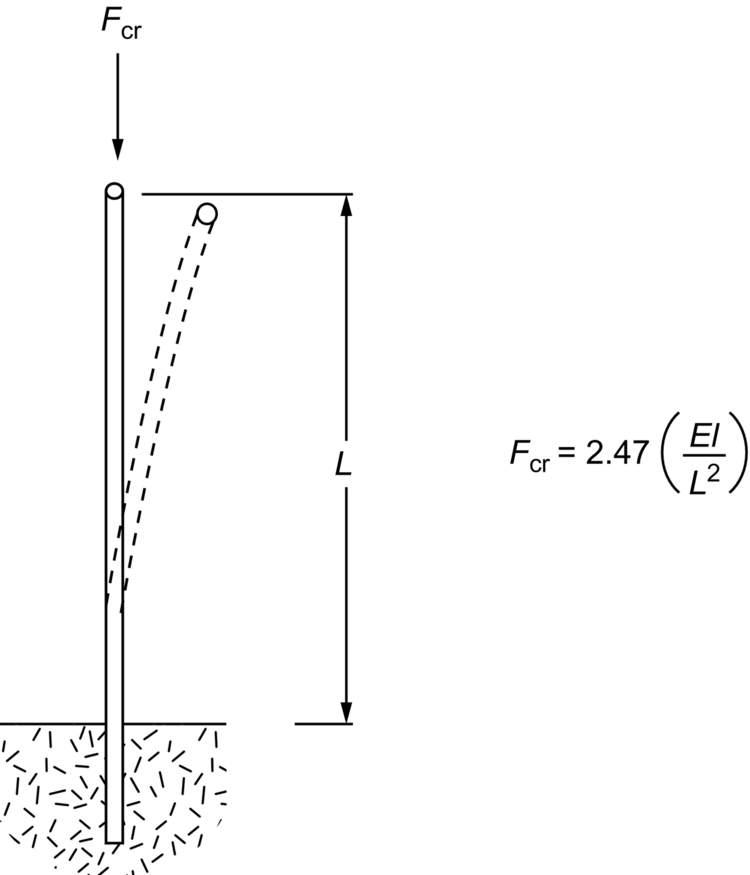
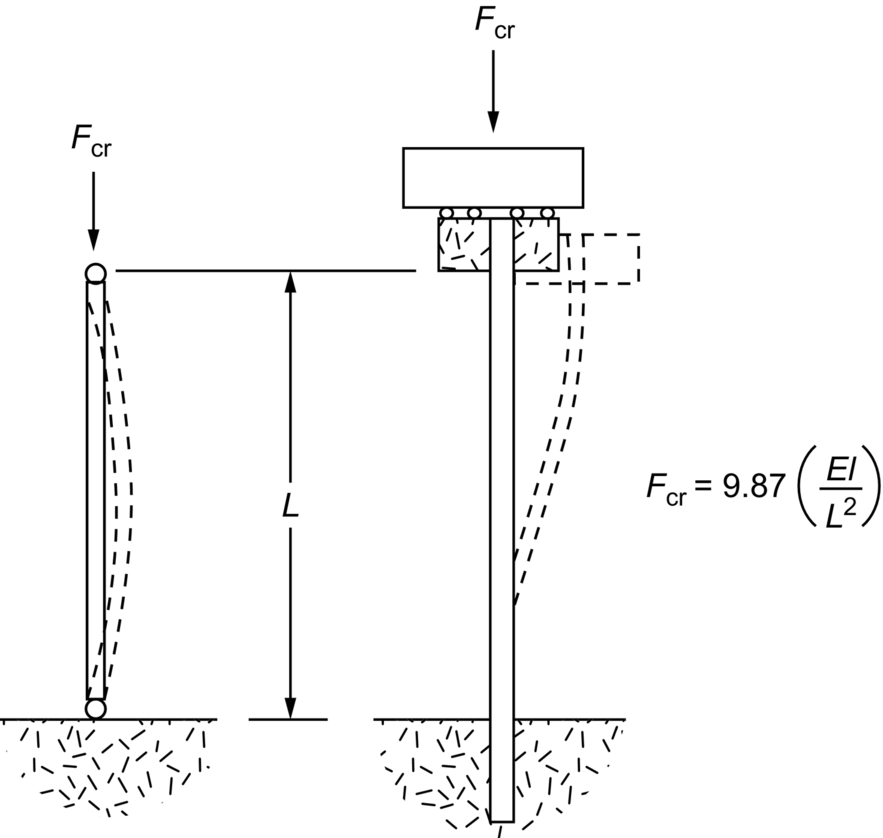
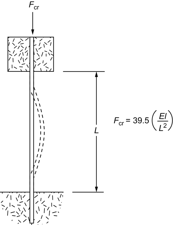
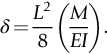
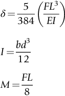
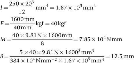
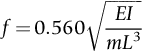
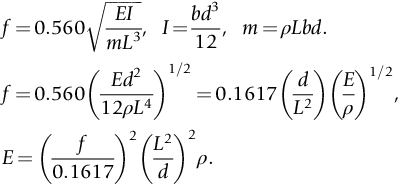
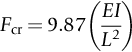
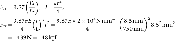
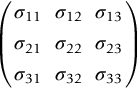
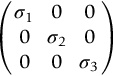
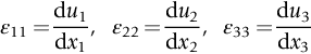
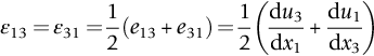
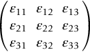
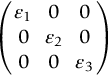
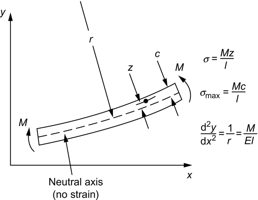
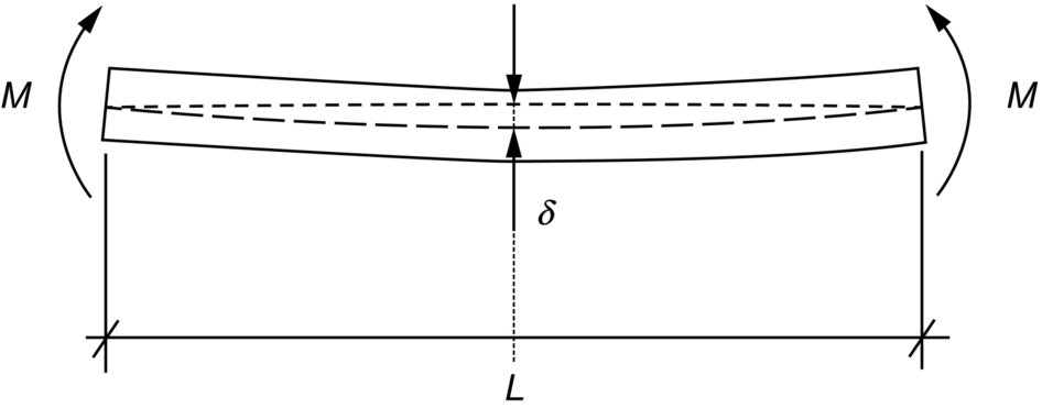
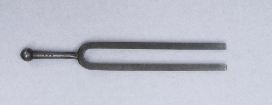
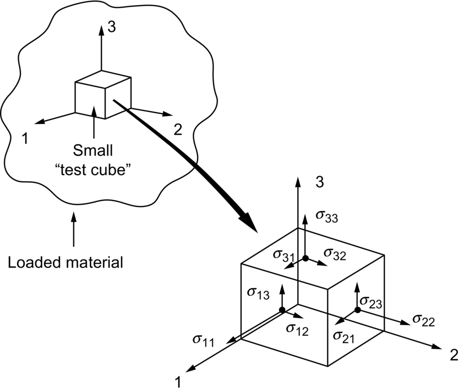
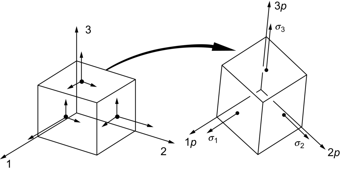
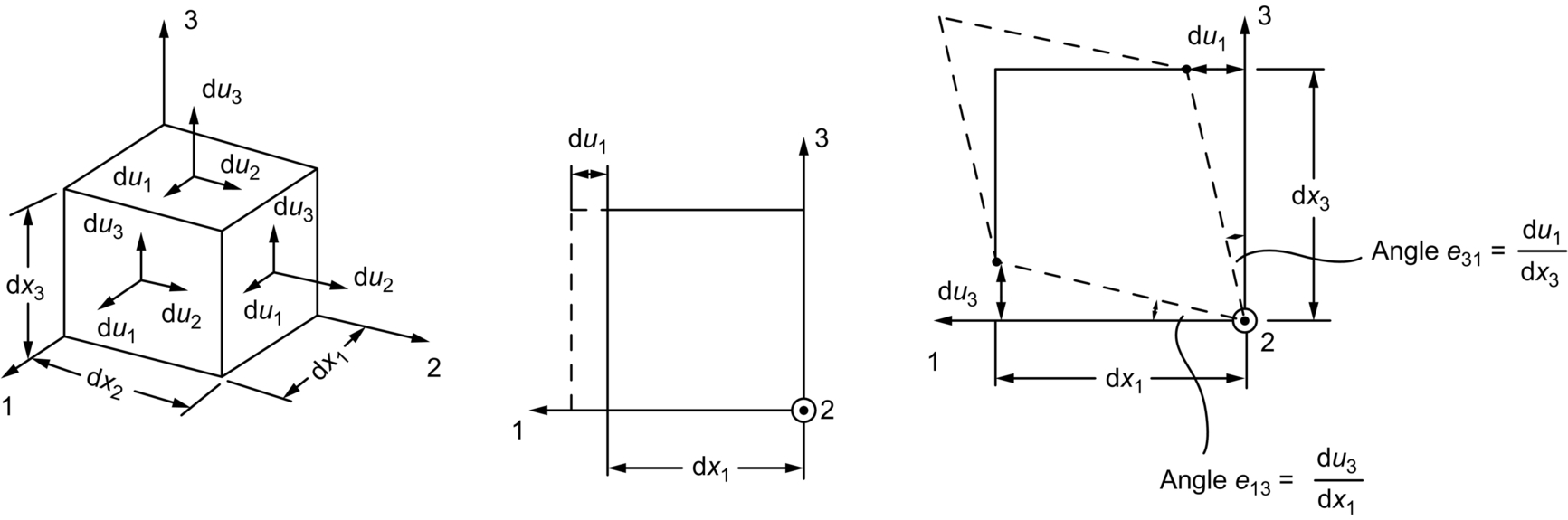
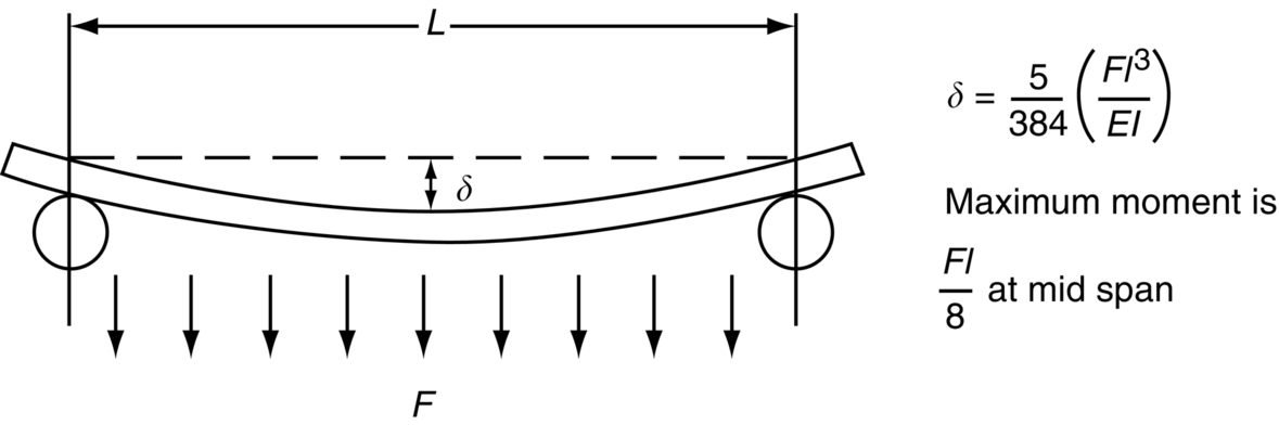
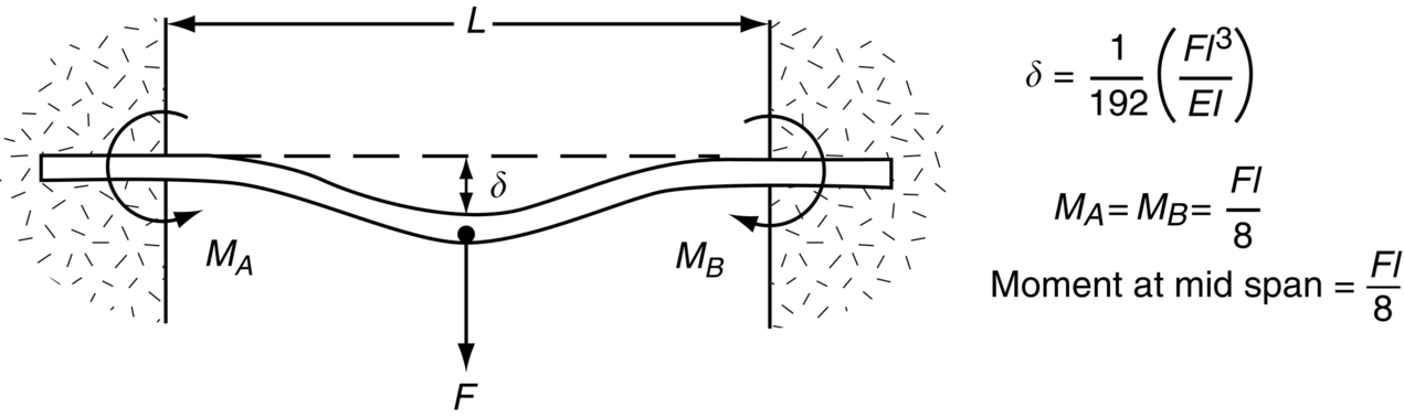
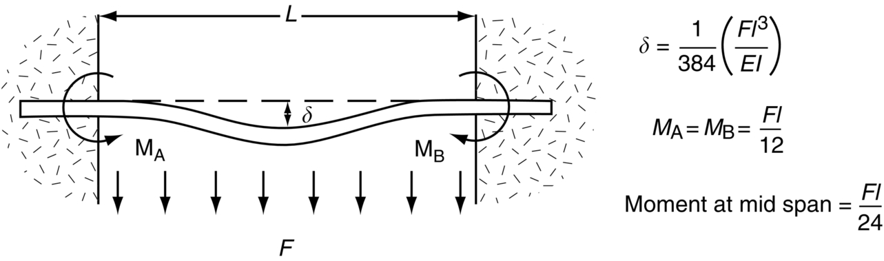
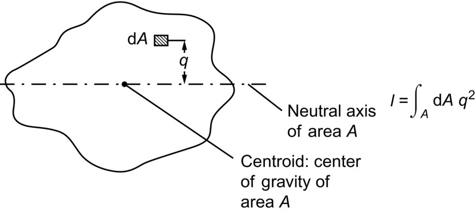
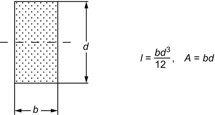
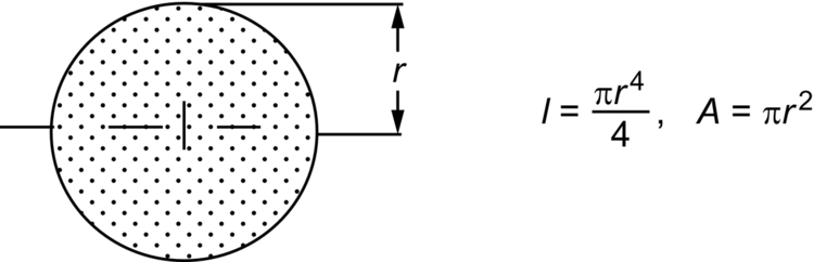
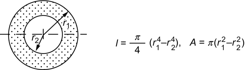
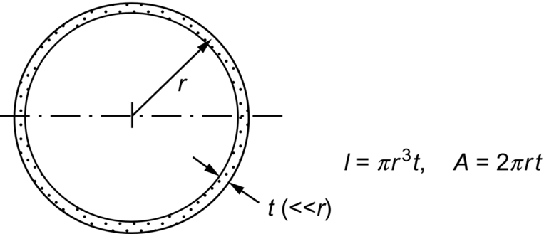
section epub:type=”chapter”> In Chapter 3, we showed that materials deform elastically, provided we stay within the elastic limit. Materials with a large modulus were stiff, and those with a small modulus were floppy. In Chapter 3, we only looked at simple applications of elastic deformation, such as the elastic extension of a bolt loaded in tension along its length (see Figure 3.4 or Figure 3.5(a)). If the bolt is made of a stiff material like steel, then the maximum elastic extension is very small, of the order of 0.1%. A strain, which is greater than this, will exceed the elastic limit. However, there are many engineering applications where a high-modulus material—which is stiff under straight loading—is anything but stiff under other forms of loading. This has important consequences for design where elastic deflection is either desirable (e.g., springs in automobile suspensions) or undesirable (e.g., bridge girders). We will look at some detailed case studies involving elastic deformation in Chapter 8. An important application of elastic deformation is elastic bending. You can see this for yourself by doing two simple tests on a plastic ruler. If you grip the ruler firmly at each end with your hands, and then pull it along its length, you will not feel any “give.” There has to be some increase in length of course, but it would need precision instrumentation to measure it. However, if you bend the two ends toward one another, the ruler will form into a curve, and the more you bend, the more it will curve. The ruler is behaving as a “beam”—and bending a beam is a very effective way of converting a very small elastic strain into a very large elastic deflection. Figure 7.1 shows what happens when you bend a beam into a radius r. The inside of the curve gets a little shorter, and the outside gets a little longer. The strain is a maximum at the surfaces of the beam and is zero at the center (the “neutral axis”). On the inside of the curve the strain (and stress) are compressive, and on the outside of the curve the strain (and stress) are tensile. Because the beam is thin, a small strain at the surfaces produces a very noticeable curvature—and if the beam is a long one, this leads to a large sideways deflection. The radius r of the beam is given by the equation where M is the “bend” at the ends (the bending moment), E is Young’s modulus, and I is a term called the second moment of area. I describes how “thin” the beam is. This equation describes exactly what you would expect—the beam bends more (r decreases) if E is small (a floppy material), or the beam is thin (small I) or you bend it a lot (large M). Figure 7.2 shows a beam of length L with a bending moment M applied at the ends. The deflection (δ) is greatest half-way along the length, and is given by the equation Equation (7.2) converts from the r of Equation (7.1) to δ and L, which are more useful for design problems. Deriving Equation (7.2) only involves simple geometry, because the value of r is the same everywhere along the length of the beam. Other ways of loading a beam are more complex, because M—and therefore r—varies along the length of the beam. Values of δ for other loading conditions are given at the end of this chapter (see the results for bending of beams). But how do we calculate I? Details are given at the end of this chapter (see the results for second moments of area). One example—for a beam with a rectangular cross section—is I = bd3/12. If you double the width b of the beam, you halve the deflection. But if you double the thickness d, you decrease the deflection by a factor of 23 = 8 times! Sian wants to keep her large collection of books in a recess in her sitting room. The recess is 1600 mm wide and you offer to install a set of pinewood shelves, each 1600 mm long, supported at their ends on small brackets screwed into the wall. You guess that shelves measuring 20 mm deep by 250 mm wide will be OK. However, professional integrity demands you calculate the maximum deflection first. For pine, E ≈ 10 GN m–2. A book 40 mm thick weighs about 1 kg. Use the results in this chapter for bending of beams, and second moments of area. The appropriate beam bending case is Case 4. Then, The shelves will deflect noticeably (12.5 mm). This deflection is just about acceptable aesthetically, but it may increase with time due to creep (see Chapter 21). One solution would be to turn the shelf over every six months. This will not be popular however, and you are better advised to increase the thickness instead. You can try this for yourself with a wooden ruler. You clamp one end of the ruler to the edge of a table, so most of the ruler overhangs the edge of the table. Then you “twang” the ruler, by deflecting the free end, and suddenly letting it go again. You can experiment by using different lengths of vibrating ruler (altering the overhang), and also by adding mass to the ruler (e.g., sticking some modeling clay on it). What you find is that the frequency of the vibration, f, goes down with increasing overhang and mass. The math analysis for a “twanged” beam fixed at one end (free length L, uniformly distributed mass m) gives Values of f for various beam constraints and mass distributions are given at the end of this chapter (see the results for vibration of beams)—they all have the same math form as Equation (7.3), and the only thing that changes is the numerical constant. But why are vibrations like this important? We have already seen one example in Chapter 6—the vibration of strips of cane in the oboe reed. Many musical instruments rely totally on the vibration of bits of cane, wood, or metal. Saxophone, clarinet, and bassoon reads are vibrating beams; so are the soundboards of pianos, guitars, and violins; or the bars of xylophones. But in the wider engineering world, often the last thing one wants is vibrations—or at least vibrations at the “wrong” frequency. They can destroy bridges, like the Tacoma Narrows bridge; damage the rotors of aero engines or steam turbines; and anyone who has a driven an automobile with failed dampers will have experienced sprung suspension units oscillating toward destruction. The photograph shows a steel tuning fork, which produces a Concert A (440 Hz, or 440 s–1) when it is “twanged.” The arms of the fork are 85 mm long, and have a square cross section of side 3.86 mm. Using this information, we want to find the value of Young’s modulus for steel. The density of steel is 7.85 × 10³ kg m–3. Use the results in this chapter for vibration of beams, and second moments of area. The appropriate vibration case is Case 2. Because the frequency of natural vibration involves a force (N) acting on a mass (kg) to give it an acceleration (m s–2), it is crucial when real numbers are put into the final equation that these basic SI units are used as follows You can try this for yourself with a plastic ruler. You place the ruler vertically with the lower end resting on a table top, then push down on the upper end of the ruler (using a book, so your hand does not get indented!). At a critical load, Fcr, the ruler starts to bow out sideways, and you have to release the force so you don’t break the ruler. The math analysis for this situation gives Values of Fcr for various beam constraints are given at the end of this chapter (see the results for buckling of beams)—they all have the same math form as Equation (7.4), and the only thing that changes is the numerical constant. Buckling is important in structural design—you may wish to support a building on steel columns, and they may be within the elastic limit when loaded in compression, but if the load equals or exceeds Fcr, then the building will collapse. It is intuitively obvious that you are more likely to get buckling if the columns are long (large L), thin (small I), and made from a floppy material (small E), and in fact that is exactly what Equation (7.4) tells us. Uncle Albert has been given an elegant hickory (hardwood) walking stick. It is 750 mm long and 17 mm in diameter (being an engineer, you always carry measuring equipment around with you). The stick is straight, and the top end terminates in a small ball-shaped handle. He is very pleased with his stick, but you have your doubts that it can support his full weight (90 kg on a good day). You need to do the calculations to see whether he will be OK. Assume that E = 20 GN m–2 (2 × 10⁴ N mm–2) for the wood. Use the results in this chapter for buckling of beams, and second moments of area. The appropriate buckling case is probably Case 2 (left-hand side drawing). Then, This gives a factor of safety of about 148/90 = 1.65, so he should be OK. Beams in bending (either deflecting, or vibrating, or buckling) have simple distributions of stress and strain, which can be calculated using classical algebraic equations. But many components have a more complex distribution of stress and strain (like the eye of the eyebolt in Figure 3.4). In order to handle stresses and strains in more complex geometries, we need a simple way to describe them in three dimensions. As Figure 7.3 shows, even though the stresses inside a loaded component may be very complex, we can express the stress state at any given position by a total of three tensile stress components and six shear stress components. The tensile stress components are σ11, σ22, and σ33. The subscripts mean “normal” and “direction,” respectively—for example σ11 is a stress, which acts on a plane, which is “normal” (at right angles) to the 1 axis, and it acts in a “direction,” which is parallel to the 1 axis. If A is the area of a cube face, and Ft is the tensile force applied parallel to the 1 axis, then σ11 = Ft/A. The shear stress components are σ21, σ12, σ31, σ13, σ32, σ23. So, for example, σ12 acts on the plane, which is normal to the 1 axis, but it acts in the direction, which is parallel to the 2 axis. If A is the area of a cube face, and Fs is the shear force applied parallel to the 2 axis, then σ12 = Fs/A. The shorthand way of writing these nine stress terms out is called the stress tensor. You may have come across tensors in math or mechanics, and learned how to manipulate them. You do not need to know anything about them here—we are simply using them as a clear way of showing the stress terms. The stress tensor is written out as The leading diagonal is the line that runs from top left to bottom right. So, the tensile stresses run down the leading diagonal in order 1, 2, 3. The shear stresses are the off-diagonal terms. The shear stresses are not all independent of one another. In fact, σ21 = σ12, σ31 = σ13, and σ32 = σ23. This means that the tensor is symmetrical about the leading diagonal. But why is this the case? Let’s look at Figure 7.3, and the shear terms σ21 and σ12. σ21 = Fs/A, and σ12 = Fs/A. The shear force Fs acting on the “2” plane tries to rotate the cube clockwise about the “3” axis. But the shear force Fs acting on the “1” plane tries to rotate the cube counterclockwise about the “3” axis. For equilibrium, the two rotational terms must balance out, and this can only happen if σ21 = σ12. It can be shown mathematically that the “test cube” can always be rotated into a particular orientation where the shear terms vanish (see Figure 7.4). In this case, the axes become principal directions (written as 1P, 2P, 3P) and the tensile stresses become principal stresses (written as σ1, σ2, σ3). The cube faces become principal planes. Free surfaces of components are always principal planes, because they cannot carry any shear stresses. The principal stress tensor is The sum of the tensile stress components stays constant when the test cube is rotated, for example σ11 + σ22 + σ33 = σ1 + σ2 + σ3. Figure 7.5 shows that we can describe strain components in a similar way to stress components—the test cube has three tensile strains and six shear strains (although there are only three independent shear strains). The three tensile strains are Each pair of equal strain components is written in the form (see Figure 7.5) The strain tensor is written out as The tensile strain components run down the leading diagonal in order 1, 2, 3, and the shear strain components are the off-diagonal terms. The strain tensor is symmetrical about the leading diagonal. The principal strain tensor is The sum of the tensile strain components stays constant when the test cube is rotated, for example ɛ11 + ɛ22 + ɛ33 = ɛ1 + ɛ2 + ɛ3. The following Examples illustrate these concepts, and in Chapter 8 we use them in a detailed case study of the Challenger space shuttle disaster. Case 1 Case 2 Case 3 Case 4 Case 5 Case 6 Case 1 Case 2 Case 3 Case 4 Case 5 Case 6 Case 1 Case 2 Case 3
Applications of Elastic Deformation
7.1 Introduction
7.2 Bending
Worked Example 1
7.3 Vibration
Worked Example 2
7.4 Buckling
Worked Example 3
7.5 Stress and Strain in Three Dimensions
Examples
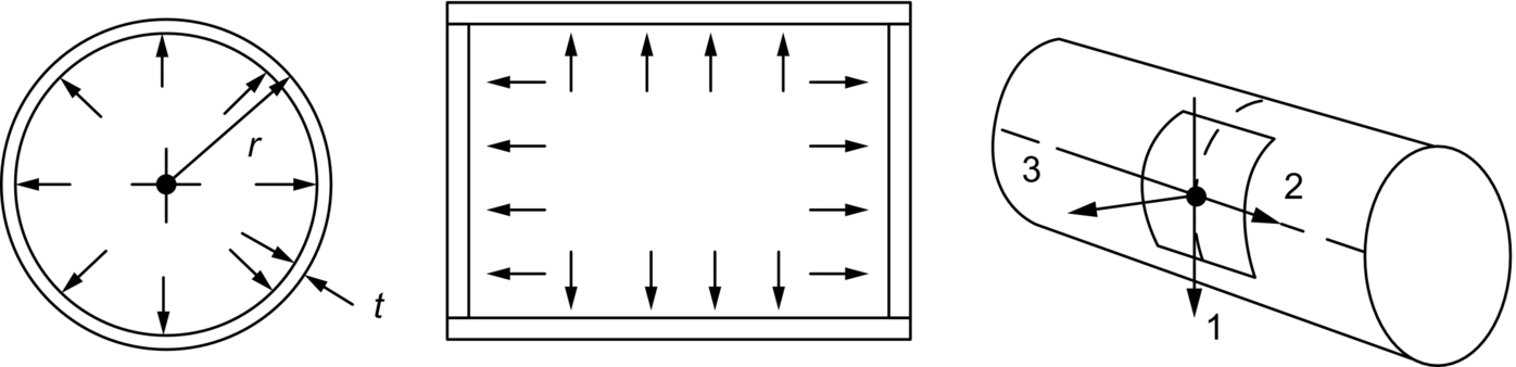
 and the longitudinal (axial) stress is given by
  . Write out the principal stress tensor for this stress state. Why must the 1, 2, and 3 axes be the principal directions?
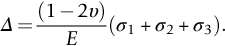
Hence derive an equation for the dilatation in terms of Poisson’s ratio, Young’s modulus, and the sum of the principal stresses. For what value of ν is the volume change zero?
[Hint—use the equation you derived for the dilatation in Example 7.11, and set each of the principal stresses equal to − p.]
Hence show that K = E when ν = 1/3.
Answers
 ,
,
(b)  ,
,
(c) 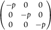 ,
,
(d)  .
.
 .
.
 . There are no shear stress components normal to these axes.
 .
.
(b)  .
.

Consider a cube of material of unit side. For each of the three principal (axial) strains, the increase in the volume of the cube is equal to the strain. For example, a strain ɛ1 makes the cube longer in the 1 direction by ɛ1. The increase in the volume of the cube is ɛ1 × 1 × 1 = ɛ1. The dilatation produced by ɛ1 is therefore (ɛ1 × 1 × 1)/(1 × 1 × 1) = ɛ1. Therefore, Δ = ɛ1 + ɛ2 + ɛ3.
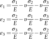
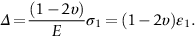
 . Now apply a stress σ2 along the 2 direction. This will produce a strain along the 2 direction of
  . In turn, this strain will produce a strain along the 1 direction of
 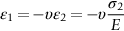 . The net strain along the 1 direction now becomes
  . Next apply a stress σ3 along the 3 direction, and repeat as before to find the total net value of ɛ1, as given by the first equation. Repeat this procedure to find the equations for ɛ2 and ɛ3. Sum the three principal strains using the three equations. It is then straightforward to show that
The dilatation is zero when υ = 1/2.
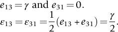
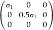
The volume changes are therefore 0.4ɛ1, ɛ1, and 0.
 . For hydrostatic pressure loading, the equation
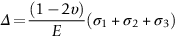 becomes
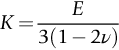
 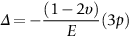 . Then
 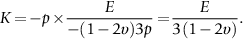 This shows that K = E when υ = 1/3.
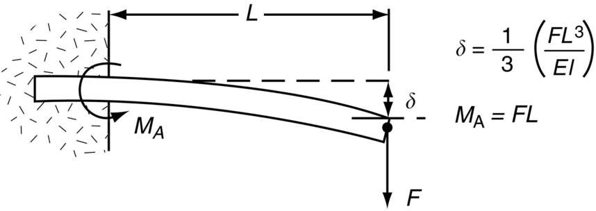
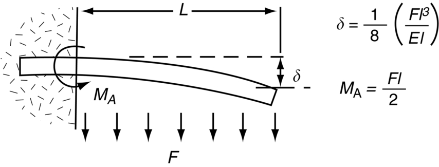
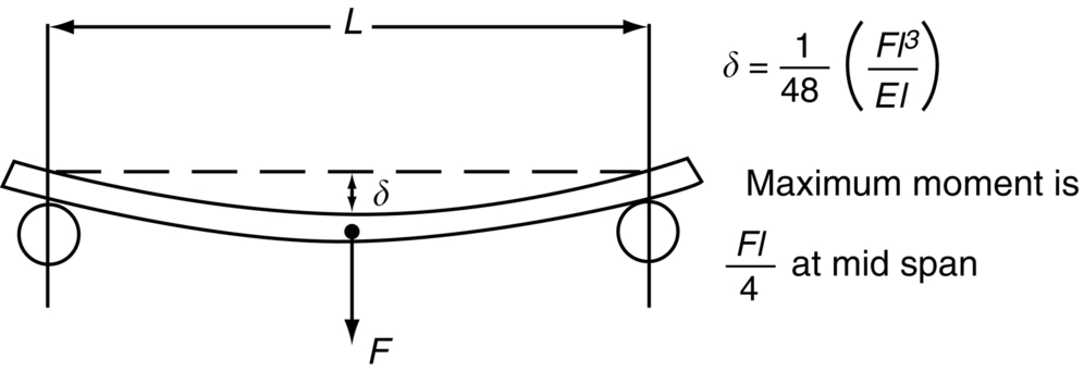
Bending of Beams
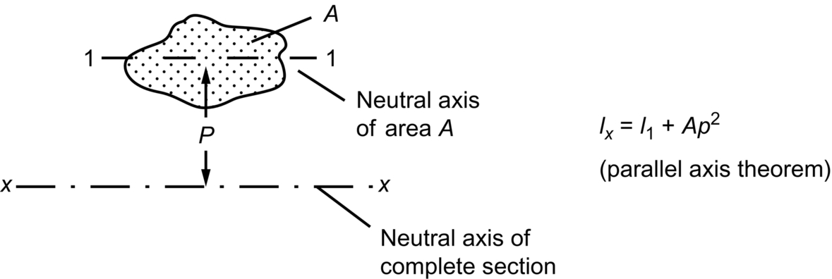
Second Moments of Area

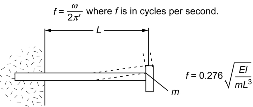
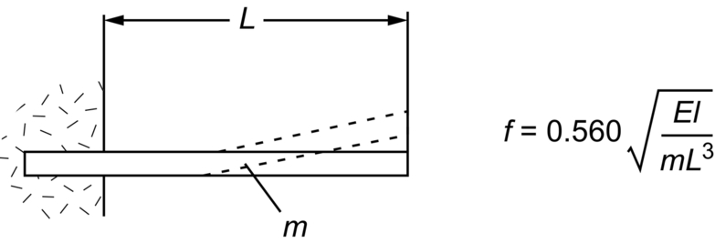
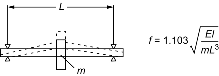
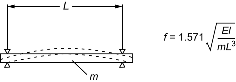
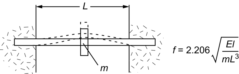
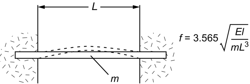
Vibration of Beams
Buckling of Beams