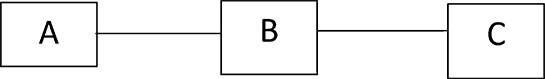
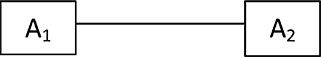
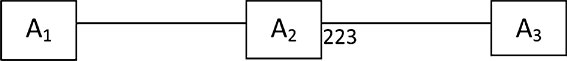
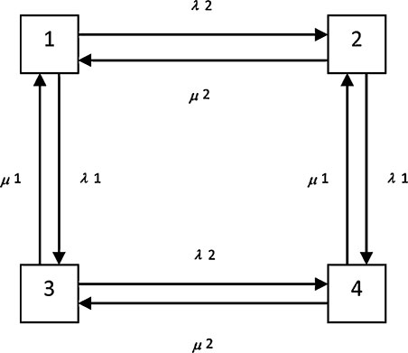
Any power plant consists of a number of generators. The present chapter presents each generator with two or more states that the generator is passing through. The generator status represented in a matrix form. To combine the generators, a special type of mathematics needed and illustrated. The matrix dimension is the form based on the generator status. The present chapter starts with the basic definitions and properties of the Kronecker product of matrices. At the same time, it should be noted that the Kronecker products have many applications such as image processing, signal processing, and other applications. In the present chapter, the Kronecker technique presented and applied to the power plant, where it is forming a power station. The Kronecker results compared with direct differentiation results. The conclusion reached with that the Kronecker product is more convenient and simpler than the direct differentiation method (Society for Industrial and Applied Mathematics, 2005).

7.2 KRONECKER MULTIPLICATION

The general rule for Kronecker multiplication shown by considering two subsystems A and B, where the subsystem is illustrated more clear later in the real cases of applications (Shakeri et al., 2016; Mariet et al., 2016; Kepner et al., 2018).

$eq377.jpg$

Then multiplication of A B defined as:

$eq378.jpg$

where: ⊗ defined as Kronecker multiplication sign

$eq379.jpg$

In the reliability study, the system is passing through two-state models or more. Therefore, it will generalize as n-number of states that represented as follows:

Let

$eq380.jpg$

and

$eq381.jpg$

Then A ⊗ B is defined as:

$eq382.jpg$

The general shape is as shown above for n number of states for both systems.

7.3 RULES AND PROPERTIES FOR KRONECKER PRODUCTS

Using the above definition of multiplication (Broxson, 2006 and Van Loan, 2000), the ensuring results can be illustrated in the coming sub-sections (Shakeri et al., 2016; Mariet et al., 2016; Kepner et al., 2018).

7.3.1 SCALAR MULTIPLICATION (SHAKERI ET AL., 2016; MARIET ET AL., 2016; KEPNER ET AL., 2018)

In the case of n is a scalar, then

$eq383.jpg$

(1)

Proof:

The (i, j)^th block of A ⊗ (nB) is

$eq384.jpg$

7.3.2 MATRIX SUM AND PRODUCTS ASSOCIATION

In the case of matrix summation associated with Kronecker multiplication, the following are the results obtained (Shakeri et al., 2016; Mariet et al., 2016; Kepner et al., 2018):

$eq385.jpg$

(2)

$eq386.jpg$

(3)

Proof:

1. The (i, j)^th block of LHS (A + B) ⊗ C is (a_ij + b_ij) C

Therefore, the (i, j)^th of RHS is

$eq387.jpg$

Since the two blocks are equal for every (i, j), the result follows.

2. The (i, j)^th block of the LHS A ⊗ (B + C) is A ⊗ (b_ij + c_ij)

Therefore, the (i, j)^th block of the other side is

$eq388.jpg$

Since the two blocks are equal for every (i, j), the result follows.

7.3.3 PRODUCT ASSOCIATION

The product of a number of matrices is presented as (Shakeri et al., 2016; Mariet et al., 2016; Kepner et al., 2018):

$eq389.jpg$

(4)

7.3.4 MIXED PRODUCT

The mixed product of a number of matrices is presented as (Shakeri et al., 2016; Mariet et al., 2016; Kepner et al., 2018):

$eq390.jpg$

(5)

7.3.5 KRONECKER SUM

Consider the two masteries A(n × n) and B(m × m), then the following (Shakeri et al., 2016; Mariet et al., 2016; Kepner et al., 2018), the Kronecker sum can be defined by the following expression:

$eq391.jpg$

(6)

where:

I_m is a unit matrix (m × m);

I_n is a unit matrix (n × n).

7.4 KRONECKER PRODUCT MODELING

Consider a power station (Shakeri et al., 2016; Broxson, 2006; Mariet et al., 2016; Kepner et al., 2018) with three generating-units as shown in Figure 7.1 and represented by the differential equation describing the subsystem (generating-unit) that can be written as:

**FIGURE 7.1** Three sub-systems (generators).

$eq392.jpg$

Let

$eq393.jpg$

(7)

where: Q(t) is an equivalent system probability; T⁽ⁱ⁾ is the transition rate matrix for i-th subsystem; P⁽ⁱ⁾ (t) is an i-th column probability vector for the i-th subsystem.

$eq394.jpg$

Consider the first term of equation:

$eq395.jpg$

Consider the second term of the equation:

$eq396.jpg$

Therefore, the equivalent system equation becomes as:

$eq397.jpg$

The summation of the transition rate matrix, the Kronecker summation becomes:

$eq398.jpg$

where:

$eq399.jpg$

which is identical to the transition rate matrix obtained in Section 7.5.1 by more means that are laborious.

7.5 SYSTEM BUILDING

Systems formed by combining a number of simpler subsystems (Shakeri et al., 2016; Mariet et al., 2016; Kepner et al., 2018). The availability of each component described by

$eq400.jpg$

However, it is often hard to derive an overall formula for the whole system from the equations describing the subsystems. Such knowledge is necessary in order to obtain an understanding of the total system structure and in particular intersection between subsystems. This is mainly attractive if one needs to introduce common mode failures.

The sub-system matrices are the first step to build the overall matrix representing a large system by an iterative procedure, which systematically, adds each sub-system to the other. The equivalent transition matrix formed from the knowledge of each sub-system failure and repair rates.

Two different methods are discussed in the present chapter. These two methods are direct differentiation and the use of the Kronecker product. Both methods are used to obtain the equivalent transition matrix (Broxson, 2006; Van Loan, 2000), which a mathematical representation of a power station in this research.

7.5.1 SYSTEM BUILDING USING KRONECKER TECHNIQUE

As stated earlier, the Kronecker multiplication is a powerful tool to build the transition rate matrix. Therefore, the Kronecker algebra can easily present any large system by combining all the sub-systems under it. Then, using Kronecker algebra in system building, a Matlab function found to use Kronecker algebra. Furthermore, this function is not within the Matlab program yet (Shakeri et al., 2016; Mariet et al., 2016; Kepner et al., 2018).

As mentioned earlier, the Kronecker sum is:

$eq401.jpg$

(8)

where:

I_m is a unit matrix (m × m);

I_n is a unit matric (n × n).

In the system building function, the size of each sub-system is 2 × 2, this came from the equation

$eq402.jpg$

So each sub-system matrix will be as of:

$eq403.jpg$

The size of the unit matrix will be 2 × 2. The overall size of the transition rate matrix can be calculated from the number of sub-systems (n) as follows:

Transition rate matrix = 2ⁿ.

Let a system contain two sub-systems A and B. Then:

Transition rate matrix = A ⊗ B = A ⊗ I_B + I_A ⊗ B

$eq404.jpg$

Then,

$eq405.jpg$

and

$eq406.jpg$

Then

$eq407.jpg$

Then the transition rate matrix for system containing two subsystems A and B are:

$eq408.jpg$

It should be noted that the Kronecker multiplication of a two-unit matrix with the same size is equal to doubling the size of the matrix, i.e., let I₁ size 2 × 2; I₂ size 2 × 2 and I₃ size 2 × 2, then

$eq409.jpg$

(9)

Proof:

$eq410.jpg$

I₁ ⊗ I₂ ⊗ I₃ =

$eq411.jpg$

Then,

$eq412.jpg$

Three sub-systems A, B, and C then the transition rate matrix equal to:

$eq413.jpg$

It is well known that the Kronecker Multiplication step:

A ⊗ I_B ⊗ I_C = A ⊗ I (where I size 4 × 4)

I_B ⊗ B ⊗ I_C =

$eq414.jpg$

Therefore, the Kronecker summation

$eq415.jpg$

where:

$eq416.jpg$

From the above examples, the Kronecker Sum can be generalized in the following equation:

$eq417.jpg$

In case, the evaluation of electric power plant is required. Therefore, the Kronecker is applied. For the different electric power plant, the reliability evaluation is required. As an example, five generators are assumed, and their data represented in Table 7.1. The results of combinations for the five generators are 32 steady-state probabilities are calculated and recorded in Table 7.2, where each generating-unit assumed to pass through two states. It should be noted that (1) means the generating-unit is ON and (0) means the generating-unit is OFF. Furthermore, it is assumed that each generator is working with its full capacity.

The calculation of the number of states that the five generators are passing through can be calculated as:

$eq418.jpg$

where:

2 represent the number of states that each generator is passing through;

5 represent the number of generators.

**TABLE 7.1** Five Generating-Units (Assumed as First Electric Power Plant)
Unit No.	Capacity (MW)	Number of Failures (Times per year)	MTTR (Hour)
1	100	3	3.770
2	100	5	9.238
3	100	6	4.045
4	100	5	6.844
5	100	4	0.570

**TABLE 7.2** Five Generating-Units Results (First Electric Power Plant)
Probability #	Unit # 1	Unit # 2	Unit # 3	Unit # 4	Unit # 5
1	1	1	1	1	1
2	1	1	1	1	0
3	1	1	1	0	1
4	1	1	1	0	0
5	1	1	0	1	1
6	1	1	0	1	0
7	1	1	0	0	1
8	1	1	0	0	0
9	1	0	1	1	1
10	1	0	1	1	0
11	1	0	1	0	1
12	1	0	1	0	0
13	1	0	0	1	1
14	1	0	0	1	0
15	1	0	0	0	1
16	1	0	0	0	0
17	0	1	1	1	1
18	0	1	1	1	0
19	0	1	1	0	1
20	0	1	1	0	0
21	0	1	0	1	1
22	0	1	0	1	0
23	0	1	0	0	1
24	0	1	0	0	0
25	0	0	1	1	1
26	0	0	1	1	0
27	0	0	1	0	1
28	0	0	1	0	0
29	0	0	0	1	1
30	0	0	0	1	0
31	0	0	0	0	1
32	0	0	0	0	0

Then, consider a second power plant representing six generating-units illustrated in Table 7.3. The results of combinations for the six generating-units are 64 steady-state probabilities are calculated and recorded in Table 7.4, where each generating-unit assumed that it is passing through two states. It should be noted that (1) means the generating-unit is ON and (0) means the generating-unit is OFF. Furthermore, it is assumed that each generator is working with its full capacity.

**TABLE 7.3** Six Generating-Units (Assumed as Second Electric Power Plant)
Unit No.	Capacity (MW)	Number of Failures (Times per year)	MTTR (Hour)
1	200	3	2.690
2	200	2	1.915
3	200	2	4.010
4	200	1	3.920
5	200	2	2.040
6	200	2	4.300

**TABLE 7.4** Six Generating-Units Results (Second Electric Power Plant)
Probability	Unit # 1	Unit # 2	Unit # 3	Unit # 4	Unit # 5	Unit # 6
1	1	1	1	1	1	1
2	1	1	1	1	1	0
3	1	1	1	1	0	1
4	1	1	1	1	0	0
5	1	1	1	0	1	1
6	1	1	1	0	1	0
7	1	1	1	0	0	1
8	1	1	1	0	0	0
9	1	1	0	1	1	1
10	1	1	0	1	1	0
11	1	1	0	1	0	1
12	1	1	0	1	0	0
13	1	1	0	0	1	1
14	1	1	0	0	1	0
15	1	1	0	0	0	1
16	1	1	0	0	0	0
17	1	0	1	1	1	1
18	1	0	1	1	1	0
19	1	0	1	1	0	1
20	1	0	1	1	0	0
21	1	0	1	0	1	1
22	1	0	1	0	1	0
23	1	0	1	0	0	1
24	1	0	1	0	0	0
25	1	0	0	1	1	1
26	1	0	0	1	1	0
27	1	0	0	1	0	1
28	1	0	0	1	0	0
29	1	0	0	0	1	1
30	1	0	0	0	1	0
31	1	0	0	0	0	1
32	1	0	0	0	0	0
33	0	1	1	1	1	1
34	0	1	1	1	1	0
35	0	1	1	1	0	1
36	0	1	1	1	0	0
37	0	1	1	0	1	1
38	0	1	1	0	1	0
39	0	1	1	0	0	1
40	0	1	1	0	0	0
41	0	1	0	1	1	1
42	0	1	0	1	1	0
43	0	1	0	1	0	1
44	0	1	0	1	0	0
45	0	1	0	0	1	1
46	0	1	0	0	1	0
47	0	1	0	0	0	1
48	0	1	0	0	0	0
49	0	0	1	1	1	1
50	0	0	1	1	1	0
51	0	0	1	1	0	1
52	0	0	1	1	0	0
53	0	0	1	0	1	1
54	0	0	1	0	1	0
55	0	0	1	0	0	1
56	0	0	1	0	0	0
57	0	0	0	1	1	1
58	0	0	0	1	1	0
59	0	0	0	1	0	1
60	0	0	0	1	0	0
61	0	0	0	0	1	1
62	0	0	0	0	1	0
63	0	0	0	0	0	1
64	0	0	0	0	0	0

7.5.2 SYSTEM BUILDING USING DIFFERENTIATION TECHNIQUE

The problem that is studied in this section is that of discussing the availability of the system of sub-systems in Figure 7.2, where r = 1, 2, ……, n represents a sub-system r. It is assumed that each sub-system S^(r) is either in a state S₁^(t), where the sub-system is working or dichotomously in second state S₂^(t), where it failed. The probability of being S₁^(t) and S₂^(t) are given P₁(t)^(r) and P₂(t)^(r), respectively.

The basic equation for the sub-system is further assumed to be:

$eq419.jpg$

The overall availability of the system depicted in Figure 7.2 and can be written as:

$eq420.jpg$

where A_n =P₁(t)⁽ⁿ⁾. These equations can be obtained by one of the two methods; the first methods is the use of differentiation and the second method is the generalized form using Kronecker product of matrices, these two methods are now described in detail (Shakeri et al., 2016; Mariet et al., 2016; Kepner et al., 2018).

To demonstrate the method and it is convenient to exemplify if first two sub-systems in Figure 7.2, each of them, which can be in one of two states given by the equation:

**FIGURE 7.2a** Two sub-systems generators.

**FIGURE 7.2b** Three Sub-Systems (Generators)

**FIGURE 7.2c** Four Sub-Systems (Generators)

**FIGURE 7.2d** n Sub-Systems (Generators)

$eq421.jpg$

Let

$eq422.jpg$

Then, differentiating the Q’s equations gives,

$eq423.jpg$

The complete system differential equation can be written as:

$eq424.jpg$

The state space-diagram for the above equation is described in Figure 7.3.

**FIGURE 7.3** The overall system state-space diagram of the two subsystems.

The overall system characterized by four states because each system can be in either of two states, which are compound from the simple two-states for each sub-system. The above method can be readily being generalized to a system containing N sub-systems. Again assuming that each sub-system is one of two states, one sees that the overall system can be described by the following two states given by:

$eq425.jpg$

One has M = (2)^N, where M is the total number of the equivalent system states of N.

7.6 APPLICATIONS

As stated earlier, the Kronecker product (Shakeri et al., 2016; Mariet et al., 2016; Kepner et al., 2018) is easier and faster the differentiation technique in forming the transient rate matrix. Let λ₁ = .1, λ₂ = .2, λ₃ = .3, λ₄ = .4 and λ₅ = 0.5, and let μ₁ =0.6, μ₂ =0.7, μ₃ =0.8, μ₄ =0.9 and μ₅ =0. The parameters were chosen to simplify the calculations. So, to build a system from two subsystems let λ = [0.1 0.2] and μ = [0.60.7] using the differentiation technique following the equations from (7.10) to (7.12) will give the following:

$eq426.jpg$

This will lead to the following matrix

$eq427.jpg$

Using Kronecker product is much simpler than the differentiation technique. The first step to using the transition rates between the states that the system is passing through to form the matrix that represents the systems. The second step is feeding the matrices to the Kronecker Sum program.

$eq428.jpg$

From the above, it can be seen that the use of the Kronecker product is much simpler and faster than the differentiation technique. Following is the sum of three, four, and five subsystems using the same technique.

$eq429.jpg$

The overall matrix for three subsystems is the following

Unit one ⊕ Unit two ⊕ Unit three =

$eq430.jpg$

Four Units = First Unit ⊕ Second Unit ⊕ Third Unit ⊕ Fourth Unit =

$eq431.jpg$

Five Units = Unit one ⊕ Unit two ⊕ Unit three ⊕ Unit four ⊕ Unit five =

7.7 NUMBER OF CONNECTED SUBSYSTEM

In this section, two, three, and four identical power generators connected to find out the steady-state probabilities of the connected generators to be connected (Shakeri et al., 2016; Mariet et al., 2016; Kepner et al., 2018). The generators have the same λ =.1 and μ =.9. Table 7.5 shows the number of generators connected and its respective P₁. Figure 7.4 represents the P₁ with a respective number of generators. On the same hand, applying the curve-fitting technique to find the most suitable formula for the relationship between the numbers of the generating-unit versus the first steadystate probability. The formula is becoming:

$eq432.jpg$

**TABLE 7.5** Steady-State Probability for Different Number of Generators
Number of Generators	First Steady-State Probability
2	0.8100
3	0.7290
4	0.6561
5	0.5905
6	0.5314

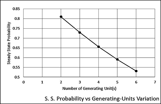
**FIGURE 7.4** First steady-state probability versus number of generators.

From Table 7.5 and Figure 7.4, it easy to see that a minimum number of connected generators illustrate the system with a lower number of generators is more reliable than that with a higher number of generating units.

KEYWORDS

• Kronecker product modeling

• Kronecker products

• Kronecker sum

• Kronecker technique

• matrix sum

• system building

REFERENCES

Broxson, B. J. “The Kronecker Product,” University of North Florida (UNF) digital commons. A Master Thesis, Submitted in Mathematics, Spring, 2006.

Kepner, J., Samsi, S., Arcand, W., Bestor, D., Bergeron, B., Davis, T., et al. Design, generation, and validation of extreme scale power-law graphs. IEEE IPDPS 2018 Graph Algorithm Building Blocks (GABB) Workshop, USA, 2018. doi: 10.1109/IPDPSW.2018.00055.

Mariet, Z., & Suvrit, S. Kronecker determinantal point processes, machine learning (cs.LG), artificial intelligence (cs.AI), machine learning (stat.ML). MIT, 2016, arXiv:1605.08374.

Shakeri, Z., Bajwa, W. U., & Sarwate, A. D. Minimax lower bounds for Kronecker-structured dictionary learning, conference: 2016. IEEE International Symposium on Information Theory (ISIT), USA, 2016. doi: 10.1109/ISIT.2016.7541479.

Society for Industrial and Applied Mathematics, 2005. Retrieved from: http://www.siam.org/books/textbooks/OT91sample.pdf (Accessed on 12 October 2019).

Van Loan, C. F. The ubiquitous Kronecker product. Journal of Computational and Applied Mathematics, 2000, 123, 85–100.

Tags: Power Systems Control and Reliability Electric Power Design and Enhancement

Aug 1, 2021 | Posted by admin in Electrical Engineer | Comments Off

7.3.1 SCALAR MULTIPLICATION (SHAKERI ET AL., 2016; MARIET ET AL., 2016; KEPNER ET AL., 2018)

7.5.1 SYSTEM BUILDING USING KRONECKER TECHNIQUE

Engineer Key

Fastest Engineer Engine

Building Power Plant

CHAPTER 7

Building Power Plant

7.1 INTRODUCTION

7.2 KRONECKER MULTIPLICATION

7.3 RULES AND PROPERTIES FOR KRONECKER PRODUCTS

7.3.2 MATRIX SUM AND PRODUCTS ASSOCIATION

7.3.3 PRODUCT ASSOCIATION

7.3.4 MIXED PRODUCT

7.3.5 KRONECKER SUM

7.4 KRONECKER PRODUCT MODELING

7.5 SYSTEM BUILDING

7.5.2 SYSTEM BUILDING USING DIFFERENTIATION TECHNIQUE

7.6 APPLICATIONS

7.7 NUMBER OF CONNECTED SUBSYSTEM

KEYWORDS

REFERENCES

Related

Fastest Engineer Engine

Building Power Plant

Share this:

Related

Related posts: