9 Computational Electromagnetic Imaging of Rough Surfaces
9.1 ROUGH SURFACES FABRICATION BY 3D PRINTING
For both the experimental target fabrication and numerical discretization, digital samples for both Gaussian and exponentially correlated rough surfaces are generated. Unlike the computer generation, it has been difficult to fabricate an exponentially correlated experimental sample by a general-purpose milling machine due to the rich high-frequency roughness. In this regard, the 3D printing technique may be applied for the fabrication. This technique allows one to directly manufacture actual samples based on the computer-generated digital sample with specific parameters, as shown in Table 9.1. More specifically, the FDM (Fused Deposition Modeling) technique is utilized for the fabrication. In this 3D printing process very thin lines of fused materials are continuously printed to construct a structure, and a 100% filling rate can be achieved to form a solid. In this way the shaping accuracy of about 0.5 mm can be achieved, which is approximately λ/20 in the Ka-band and sufficient for the imaging study. The main advantage of this technique is that it permits the usage of lossy material, to generate samples simulating the half-space rough surface scattering scenario, such as the moist soil ground. In this work, the measured permittivity is 6.22-j2.86 at 32 GHz, and that value was used in the computations of the scattering field. Figure 9.1 shows the CAD model and fabricated samples for Gaussian (a) and exponentially (b) correlated rough surface; top panel: CAD model; bottom panel: Fabricated sample. As should be noted, the considered sample has rich high frequency roughness, which generates numerous local scatters, leading to the strong speckle effects.
TABLE 9.1
Parameters of the Rough Surface Samples
| Size | RMS Height | Correlation Length | |
| Measured Sample | 250 mm in diameter | 4 mm | 48 mm |
| (in λ @ 32 GHz) | (26.7 in diameter) | (0.427) | (5.12) |
| Numerical Samples | 125 mm × 125 mm | 2 mm, 4 mm, 8 mm, 12 mm | 48 mm |
| (in λ @ 32 GHz) | (13.3 × 13.3) | (0.214, 0.427, 0.854, 1.281) | (5.12) |
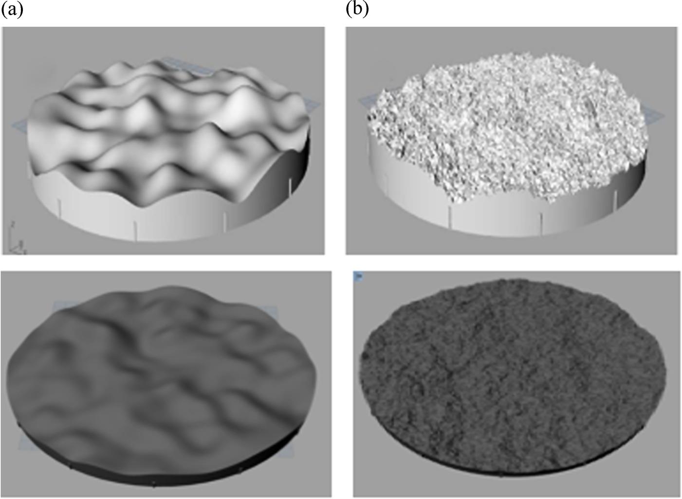
FIGURE 9.1 Geometry Configuration of the 3D model and the fabricated sample of the Gaussian (a) and exponentially (b) correlated rough surface. Top: CAD model; Bottom: Fabricated sample.
To study the speckle properties, we need a large number of computer-generated surface samples. An exponential correlation function for the random rough surface is taken since it describes better the natural ground surface [1]. In this context, the following procedures are excised: first, a very large rough surface mesh is generated on grids, then the digital sample for each realization (400*400 meshing points) is cut from that large mesh. In the cutting, one sample is neighboring and overlapping to next with 100 discretize interval (100*interval size~31 mm) distant, which is close to the footprint size in diameter in the numerical simulations. For the speckle study, 1600 (40*40) samples are obtained for one to achieve an enough number of realizations. The digital samples are then input into the FDTD simulator one by one for computing scattering in the 3D computational domain.
In the context of radar imagery, understanding the speckle properties is imperative for both image de-noising and applications such as land-cover classification and parameter retrieval [1–4]. Radar speckle arises due to the coherent sum of numerous distributed scattering contributions [4]. A general assumption is the “fully developed” speckle model, which is applicable when the resolution cell size is much larger than the correlation length () of the ground surface [4]. This requirement may be met in low-to-medium image resolution. The fully developed speckle model is based on the following two hypotheses: (1) total scattering is contributed by independent scatters; (2) there is a sufficiently large number of scatters contributing to a resolution cell so that a complex Gaussian distribution is followed. For VHR radar images, these assumptions are no longer valid.
Radar backscattering and its speckle statistic variation with the resolution cell size or antenna footprint has been a subject of interest in rough surface scattering [5–9]. In [5], the convergence of backscattering coefficients versus footprint size was studied by 1-D method of moment solution. By theoretical models and indoor SAR experiments in EMSL [6,7], the dependence of polarimetric backscattering characteristics from Gaussian correlated rough surfaces on the SAR resolution cell size was examined, while the SAR images of rough soil surfaces were measured in EMSL [8]. That work includes results and analysis on the backscattering coefficients and image probability density functions (PDF), versus different resolution cell size. As the radar image resolution reaches evolves from tens of meters to approximately one meter, or even a smaller size, this topic becomes more important currently for land observations. To model high-resolution speckle properties, Di Martino et al, proposed the predicting method for the equivalent number of scatterers within the resolution cell [9], considering stochastic stationary rough surface description, and more advanced, fractal surface models. In this work, we address the topic of very high-resolution (VHR) radar speckle statistics using indoor SAR experiments and supporting full-wave simulations.
Since the prediction for the equivalent number of scatterers has been established in [9], it is used as an evaluating tool in this work. To be specific, the exponentially correlated rough surface is considered, due to its rich high-frequency roughness on the surface-air interface that leads to numerous local scattering contributions. In particular, the 3-D printing process was used to fabricate the sample surface that is used for scattering measurement conducted at Ka-band. In this manner, the image resolution scale close to the rough surface correlation length can be achieved, namely, the image resolution cell size can be at the same scale of the surface geometric undulation. In this view, the scattering mechanism from an exponentially correlated rough surface is similar to that from the sea surface, where the scattering process from short scale roughness is modulated by relatively long scale undulation [10,11]. The prediction for the equivalent number of scatterers per resolution cell from [9] is served as a reference in the analysis. Meanwhile, based on the results from experimental and supporting numerical practices considering different incident directions, the effects of scattering scale on the speckle properties can be observed. Further numerical studies are conducted with different RMS height, for discussions on both the factors of the equivalent number of scatterers and the scattering scale effects.
9.2 EXPERIMENTAL MEASUREMENTS AND CALIBRATION
In the scanning measurement, the scattering signals were captured through the antennas and microwave transceiver all along the scanning track and all over the Ka-band in a microwave anechoic chamber as shown in Figure 9.2. Before we proceed with the data acquisition, system calibration is required., as we have already introduced in section 3.42 of Chapter 3. The procedures for polarimetric calibration have been available and well documented in numerous papers [12–16]. We present a general polarimetric calibration technique using hybrid corner reflectors. We deploy only one trihedral and two dihedral corner reflectors with different rotation angles for polarimetric calibration. It is simple and makes no assumptions.
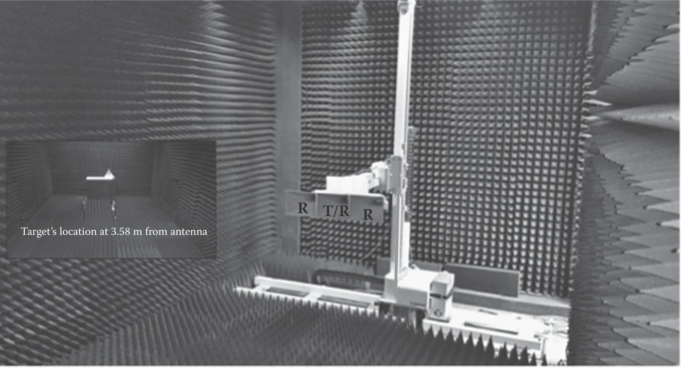
FIGURE 9.2 Measurements at microwave anechoic chamber.
In a real system, under non-ideal conditions, such as polarization cross-talk errors and channel imbalance between transmitter and receiver, the polarimetric calibration is required. This is illustrated in Figure 9.3, where and are the horizontal and vertical polarization components of the incident field, and are the horizontal and vertical polarization components of the scattered field; , , , represent channel imbalance and , , , stand for cross-talk. The wave propagation in transmitting and receiving causes the target scattering matrix distorted to a measured scattering matrix. The goal of the polarimetric calibration is to invert the target scattering matrix from the measured one to obtain a minimum difference. Propagation matrices and noise matrix are acquired from the known and reference targets. We detail the approach to obtaining the matrix elements using the calibration or reference targets as follows.
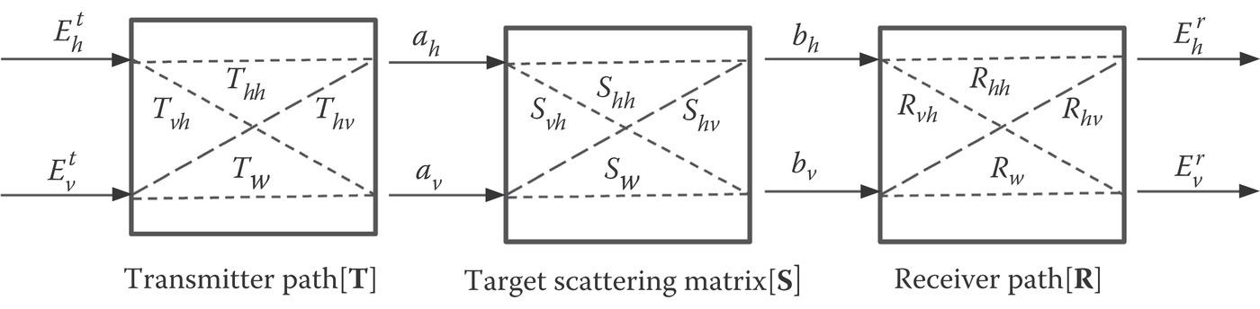
FIGURE 9.3 The process for measuring the target scattering matrix.
Referring to Figure 9.3, in a polarimetric SAR, the measured scattering matrix and true scattering matrix are related by:
where and are the true and measured 2 × 2 scattering matrices, respectively, and represent the transmitting and receiving distortion matrices, respectively, and accounts for random noise. To simplify the numerical calculation, via absorbing all possible elements of and into one matrix without considering the noise contribution involving the scattering reciprocity theorem, Equation 9.1 can be further expressed as follows:
where
The matrix is called the calibration matrix, which contains all distortion in the transmitter and receiver of the polarimetric SAR system. Using eight m matrices in place of the eight matrices, with eight unknowns are given in Equation 9.4:
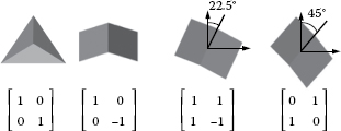
A total of eight complex unknowns in the calibration matrix need to be solved related to the co-polarizations and cross-polarizations. Therefore, we need at least two calibration targets for co-polarization and one for cross-polarization, forming eight independent complex equations for eight unknowns. In viewing six unknowns for co-polarization, and two unknowns for cross-polarization, passive corner reflectors (CR) are sufficient. They provide more convenient tracking and identification of error sources, if they occur, in the whole wave propagation process. Given these constraints, a trihedral and dihedral corner reflector constitute two equations in co-polarizations, a 45°-rotated dihedral corner reflector makes up two equations in cross-polarization, and a 22.5°-rotated dihedral corner reflector forms four equations in full polarization. Note that the rotation is about the radar incidence plane. The theoretical scattering matrices for the above-selected reflectors are listed in Table 9.2.
TABLE 9.2
Selected Corner Reflectors and Typical Scattering Matrices
 |
Based on the theoretical scattering matrices of reference targets, one trihedral and one dihedral are used to solve for the six unknown matrices (, , , , , ), which are connected with co-polarization. The solutions are given in Equation 9.5:
where .. represents the element of the measured scattering matrix of a trihedral corner reflector and similarly denotes the element of measured scattering matrix of a dihedral corner reflector. One 22.5°-rotated dihedral is used to work out the two unknowns (, ), which are related to cross-polarization. The solutions read
where denotes the element of the measured scattering matrix of a 22.5°-rotated corner reflector. After the matrix is determined, the calibrated scattering matrix can be readily obtained from
We employ three reference targets with known measured scattering matrices , and for the polarimetric calibration. We can make use of the relationship between measured and theoretical scattering matrices of reference targets to solve the calibration matrix. After the calibration matrix is determined, the scattering matrices of the reference targets can be calibrated. It follows that the scattering matrices of unknown targets can be calibrated. To assess the accuracy of the proposed calibration technique, the calibrated amplitude and phase error is calculated according to
where represents the calibrated scattering matrices of point targets, and represents the theoretical scattering matrices of point targets.
Another good measure of calibration quality is the calibrator’s polarimetric response, which is a way of visualizing the target scattering properties. We compare the polarimetric responses of the corner reflectors before and after calibration.
9.3 DATA ACQUISITION AND IMAGE FORMATION
To achieve the rough surface imaging in the chamber, the measurements are performed in the Ka–band considering the physical size of the sample prepared in section 9.1. Different bandwidths and synthetic aperture lengths were selected to achieve different spatial resolutions (in ground range), as concluded in Table 9.3. During the image processing, the Kaiser window (β = 2.5) was utilized along with the frequency and aperture signal, and the resolution cell size in Table 9.3 are realized in the presence of the Kaiser window.
TABLE 9.3
Imaging Parameters for Different Resolution Cell Size (Ground Range Resolution, Kaiser Windows ( β = 2.5) Applied in Both Domains)
| Ground Resolution | Center Frequency | Aperture Length | Bandwidth (GHz) | |||
| 30 × 30 mm2 | 32.0 GHz | 240 mm | 11.00 | 8.25 | 6.60 | 6.15 |
| 45 × 45 mm2 | 160 mm | 7.35 | 5.50 | 4.40 | 4.10 | |
| 60 × 60 mm2 | 120 mm | 5.50 | 4.13 | 3.30 | 3.07 | |
| 75 × 75 mm2 | 96 mm | 4.40 | 3.30 | 2.65 | 2.45 | |
| 90 × 90 mm2 | 80 mm | 3.70 | 2.75 | 2.20 | 2.05 | |
Detailed configuration parameters include: the track span (L) is 800 mm with an interval of 8 mm; the distance between the target scene center and the antenna (T/R) is approximately 1400 mm; the transmitting and receiving antennas are of 20 dBi gain with a half-power beam angle of 17°. In the implementation, the height difference H and distance D can be varied accordingly to achieve the beam direction or incident direction angle of 30°, 40°, 50°, and even 60°. The target is placed on a low-scattering supporting cylinder made ofthe foam material, which is set on a motor-driven rotation platform. Multiple image acquisitions should be achieved for the speckle statistics. More specifically, in each case of , the imaging measurements for the rough surface sample are performed 20 times, and after each time turntable is rotated with an equal angular interval. Therefore, 20 images are obtained for a specific , then speckle statistical analysis can be conducted based on those results.
Figure 9.4 displays radar image of rough surfaces with different resolutions of 1.5 cm, 3.0 cm, 6.0 cm, 9.0 cm in both range and azimuth directions (from top to bottom): left panel: Gaussian correlation; right panel: Exponential correlation. Only VV polarization is shown. The images were focused by the Omega-K algorithm. Finer resolution reveals subtler and detail of the scattering centers, and comparatively, in this regard, exponentially correlated rough surface contains much more fine structures that are responsible for the radar returns, or physically equivalently, the speckle strength. In fact, such phenomena have been numerically studied and confirmed from the field observations.
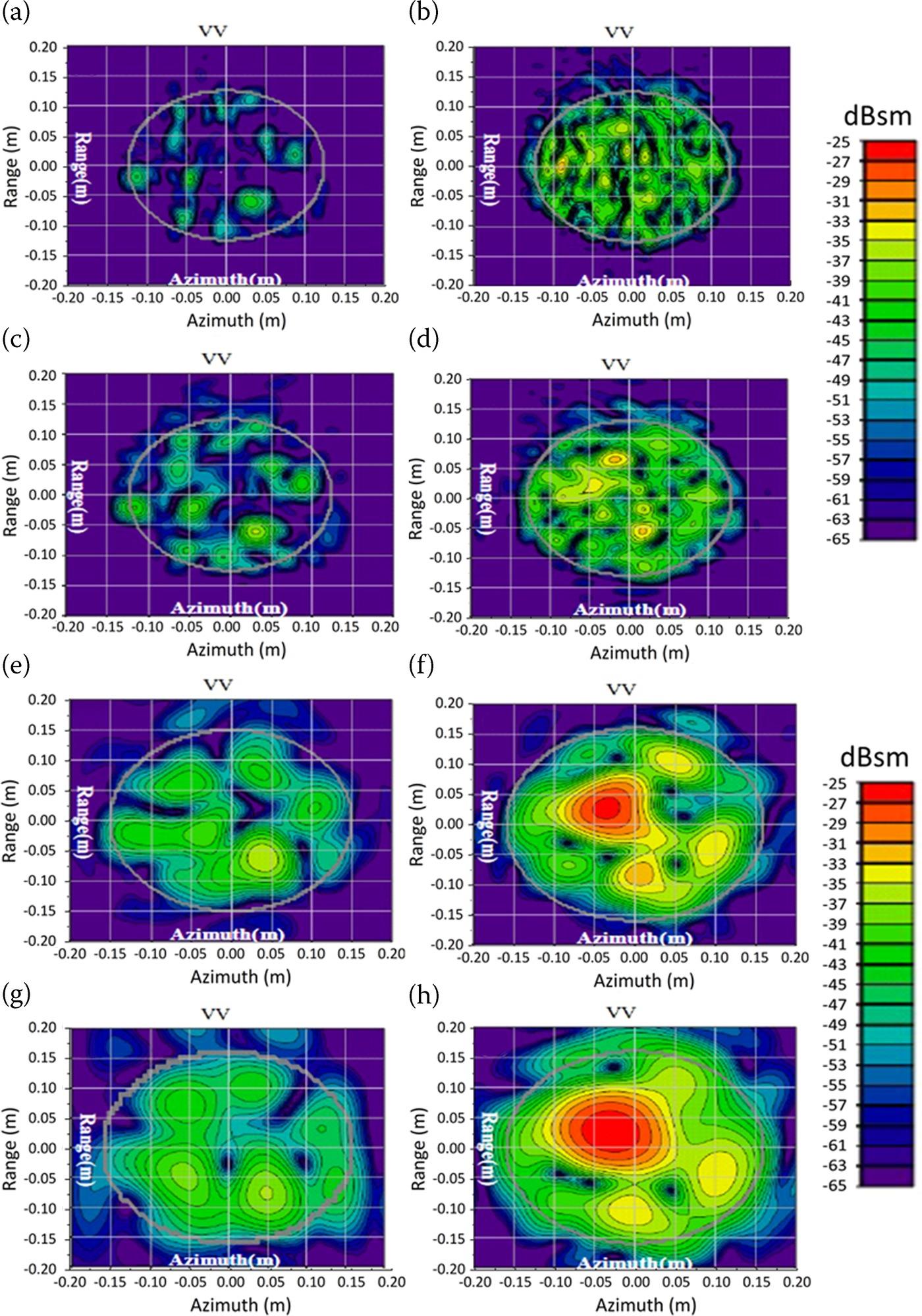
FIGURE 9.4 Radar images of rough surfaces with different resolutions of 1.5 cm, 3.0 cm, 6.0 cm, 9.0 cm in both range and azimuth directions (from top to bottom) @ VV polarization: left panel: Gaussian correlation; right panel: Exponential correlation.
After the images from the rough surface were processed, calibrated, and compensated, the amplitude speckle results were obtained for the VHR radar speckle analysis.
Although the experimental study is the most straightforward and reliable approach, it is restricted by the actual rough surface sample in both the aspects of number and size. On the other hand, the full-wave full-3D Finite Difference Time Domain (FDTD) simulator provides complementary and extensible data support. This numerical method has been reported in computing scattering from layered and heterogeneous rough surfaces [17,18]. The FDTD simulator used in this work is developed based on that reported in [19] which is a full-3D simulator, and by performing simulations on a large number of samples (realizations) one can get the backscattering results for speckle analysis as well as averaged scattering coefficients.
Figure 9.5 shows the simulation configuration in each realization, which is a typical scene for the half-space scattering. In general, the tapered incident beam is injected by the Total Field/Scatter Field boundary (TF/SF), below that boundary the incident beam immerges to illuminate the rough surface, and above that the boundary scattered field can be extracted. The Huygens Aperture collects the recorded near-field scattered field and turns that into far-field results like scattering coefficients. On the other hand, the Perfect Matching Layer (PML) is used to truncate the computation domain without introducing disturbing reflections.
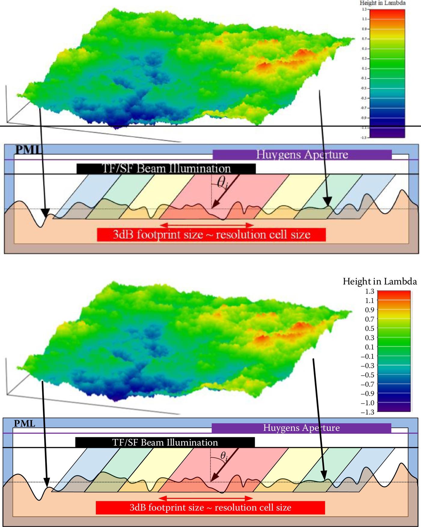
FIGURE 9.5 Configuration of FDTD simulations for rough surface scattering (The presented profile is one of realizations conducted in the numerical simulations).
Here, as a common practice, a tapered wave with a fixed ground footprint is set for the illumination. In each realization, the incident beam points to the center of the rough surface for different incident angles of 30°, 40°, and 50°. Furthermore, different surface RMS heights are also considered. The discretization cell size in the FDTD simulation is set to 1/30λ at 32 GHz, which is sufficient in modeling the high-frequency roughness of the exponentially correlated rough surface.
In general, the aim of this simulation work, which is similar to that reported in [1], is to investigate speckles by counting backscattering far-field amplitude results over a large number of realizations. The difference is that we focused on the VHR situation, which means we used a smaller tapered wave illumination region than those in the general rough surface scattering simulations. Specifically, the simulated resolution cell size is defined by the beam footprint in the numerical studies, realized by setting the footprint size equal to the required value (30 mm in diameter for 3 dB edge power drop). The detailed computation parameters are summarized in Table 9.4, and these simulations are performed to support the conclusions drawn from the VHR radar imaging experiments with a 30 mm resolution as well as further discussions. denotes the discretizing interval in the computation domain. The simulations were run on a 2-way Intel Xeon workstation with octal channel memories with each realization taking less than 5 min.
TABLE 9.4
Computational Parameters for the FDTD Simulations @ 32 GHz
| Set 1 | 3 dB Footprint Size | (mm) | Domain Size (Yee cells+) | Realization number | () |
| 30 mm in diameter | 0.3123 | 400 × 400 × 180 | 1600 | 30°, 40°, 50o | |
| Set 2 | 3 dB Footprint Size | (mm) | Z Direction Size (Yee cells) | Realization number | (mm) |
| 30 mm in diameter | 0.3123 | 160, 180, 220, 280 | 1600 | 2,4,8,12 |
Notes:
We now compare the measured scattering coefficient from the fabricated experimental sample and the model prediction by AIEM model. First, to validate the fabricated sample for the experimental imaging tests, we directly measured its scattering coefficients without the imaging process. Since in the scattering coefficient measurement only one data sample can be obtained through one measurement; apparently, sufficient ensemble samples are needed to estimate the mean value of the scattering coefficient. It turns out that more than 48 sets of backscattering data were acquired by rotating the turntable with a pedestal supporting the rough surface under measuring. Recalled that the rough surface is isotropic. Hence, the rotation of the sample generates independent ensembles as long as the sample is within the same antenna footprint. Then the backscattering coefficient data were derived according to Equations 3.39~3.43 in Chapter 3. Also, the backscattering coefficient at VV polarization derived from the calibrated image of the resolution of 60mm. The measured scattering coefficients are compared with the AIEM model predictions at different ; clearly, a good agreement can be observed in the Figure 9.6.
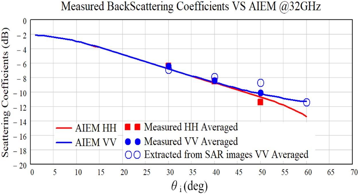
FIGURE 9.6 Comparison between measured scattering coefficients ( ) of the exponentially correlated rough surface sample, and the results by AIEM prediction, at 32 GHz.
To validate the FDTD simulation, the computational domain was increased to 1200 × 1200 × 180 Yee cells in the domain size, so as to obtain a converged scattering coefficient. In other words, the rough surface aperture size was increased to 40λ × 40λ. It should be noted that in common scattering simulations for rough surfaces [1], the aperture size of 32λ × 32λ is electrically large enough. Because of the enormous computational burden – with one realization requiring approximately 1 hour, only 50 realizations are performed to obtain the averaged scattering coefficients distributions over the upper hemisphere. Again, the AIEM results are utilized as a reference, and two sets of results are compared in Figure 9.7. Although the FDTD results failed in presenting a smooth contour due to the insufficiently large realization number, the results by numerical and analytical methods clearly agree well with each other in the overall angular patterns in the whole bistatic scattering plane.
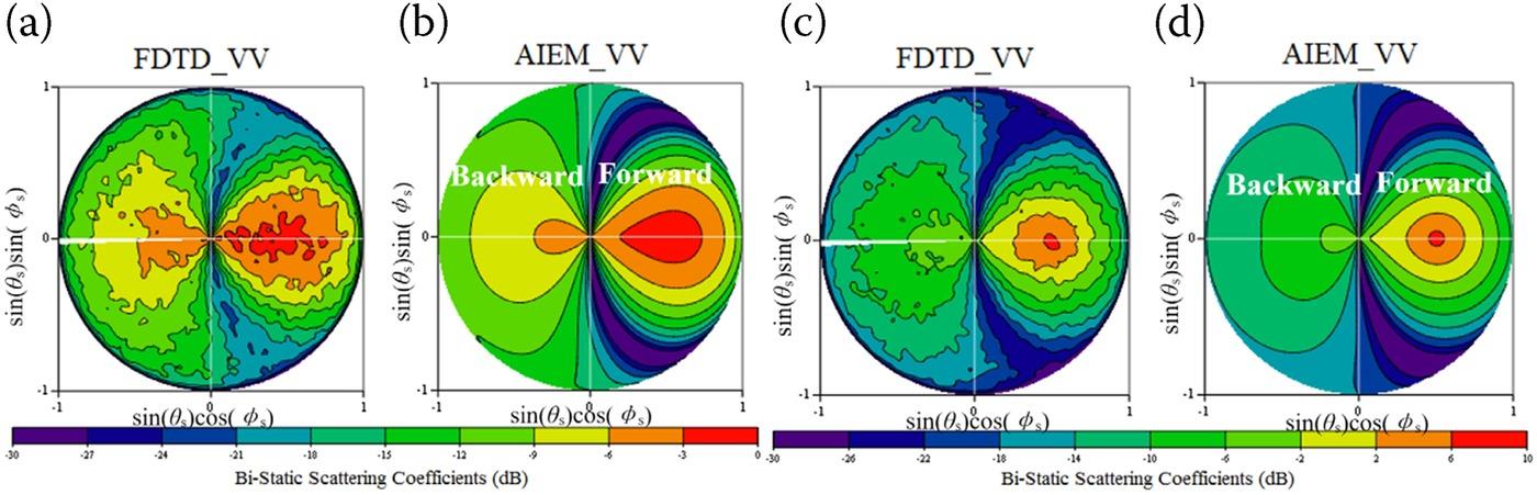
FIGURE 9.7 Comparisons between FDTD simulated upper hemisphere bistatic scattering coefficients (σ°) and AIEM results, VV, 32 GHz, exponentially correlated rough surface, relative permittivity: 6.22-2.86j; (a) and (b): correlation length l = 48 mm, RMS height σ = 4 mm; (c) and (d): l = 24 mm, σ = 2 mm.
9.4 IMAGE STATISTICS AND QUALITY
Now, based on the measured images and the simulated backscattering returns, the speckle properties can be obtained. First, the probability density function (PDF) can be computed for the amplitude and compared to the known distribution models, in particular, Rayleigh and K-distribution models. As already noted in Chapter 6, the shape factor coefficients. A larger α will push the K-distribution closer to the Rayleigh distribution that describes the fully-developed speckle. The α value for the K-distribution fitting is obtained from Equation 6.7 up to the fourth order moment of the amplitude or second-order moment of mean normalized intensity. The speckle strength at L-look data can also be readily obtained by Equation 6.4.
We now present the imaging results from the rough surface sample, the image amplitude speckle statistics, and the numerical results. In Figure 9.8, the image examples of the exponentially correlated surface are presented at different resolution scales and different values of . The scattering hot-spots at a VHR scale are observed to be fused into those at the lower resolution scales. In addition, clearly, as increases, the RCS of those spots decreases. The presented images are obtained at one of the 20 angular positions, and along with the results at other angular positions, they are used to produce the speckle results.
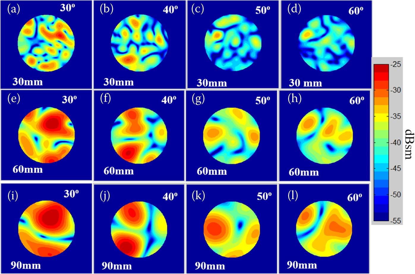
FIGURE 9.8 Image example of the exponentially correlated rough surface sample at different resolutions (30 mm, 60 mm, and 90 mm) and different (30°, 40°, 50°, and 60°), VV.
In Figure 9.9 and Figure 9.10, the image amplitude PDFs are plotted and compared to the Rayleigh distribution and the fitted K-distribution. In each sub-figure of Figure 9.9, the fitted α for the K-distribution is marked, where the resolution cell size is set to 30 mm (in azimuth and ground range), or in correlation length, 0.63l. Clearly, at the smallest of 30°, the fitted α is the smallest and the PDF curve is with the tail in semi-log plot most away from the Rayleigh curve. This fact is also observed in Figure 9.10, the results in which are with a resolution cell size of 60 mm, or in correlation length, 1.25l. Meanwhile, as the resolution cell size enlarges from 30 mm to 60 mm, the fitted α of K-distribution at each gets larger and the corresponding PDF is closer to the Rayleigh reference. That agrees with the common sense. On the other hand, it should be noted that the PDFs in the case of resolution cell size 60 mm (Figure 9.10) is not fitting the K-dis as well as those in the case of resolution cell size 30 mm (Figure 9.9). That is due to the limited size of the sample (250 mm in diameter), as it becomes insufficient in providing a good number of scatter returns with increasing resolution cell size.
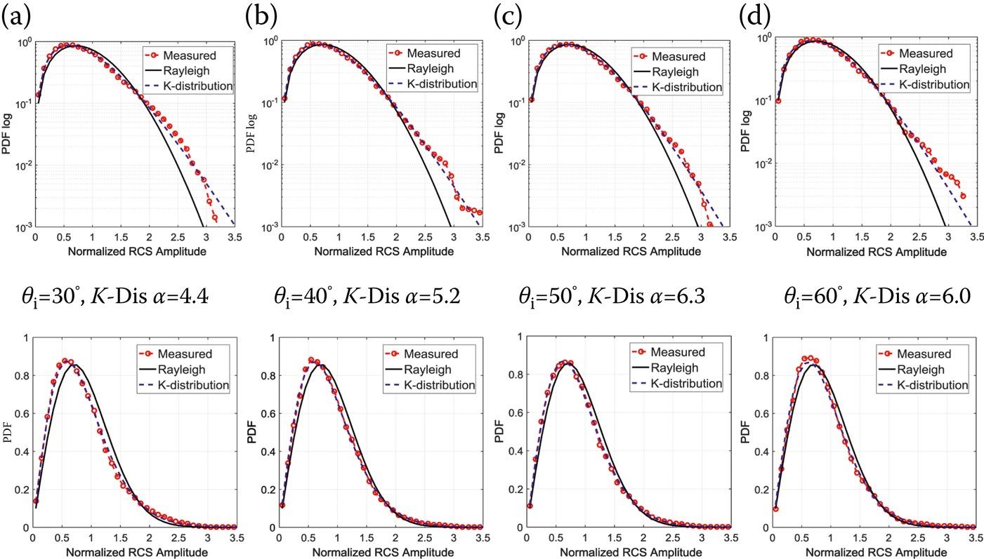
FIGURE 9.9 The normalized amplitude PDF curves of measured images at different , at the resolution cell size of 30 mm, VV, compared with Rayleigh distribution and K-distribution.
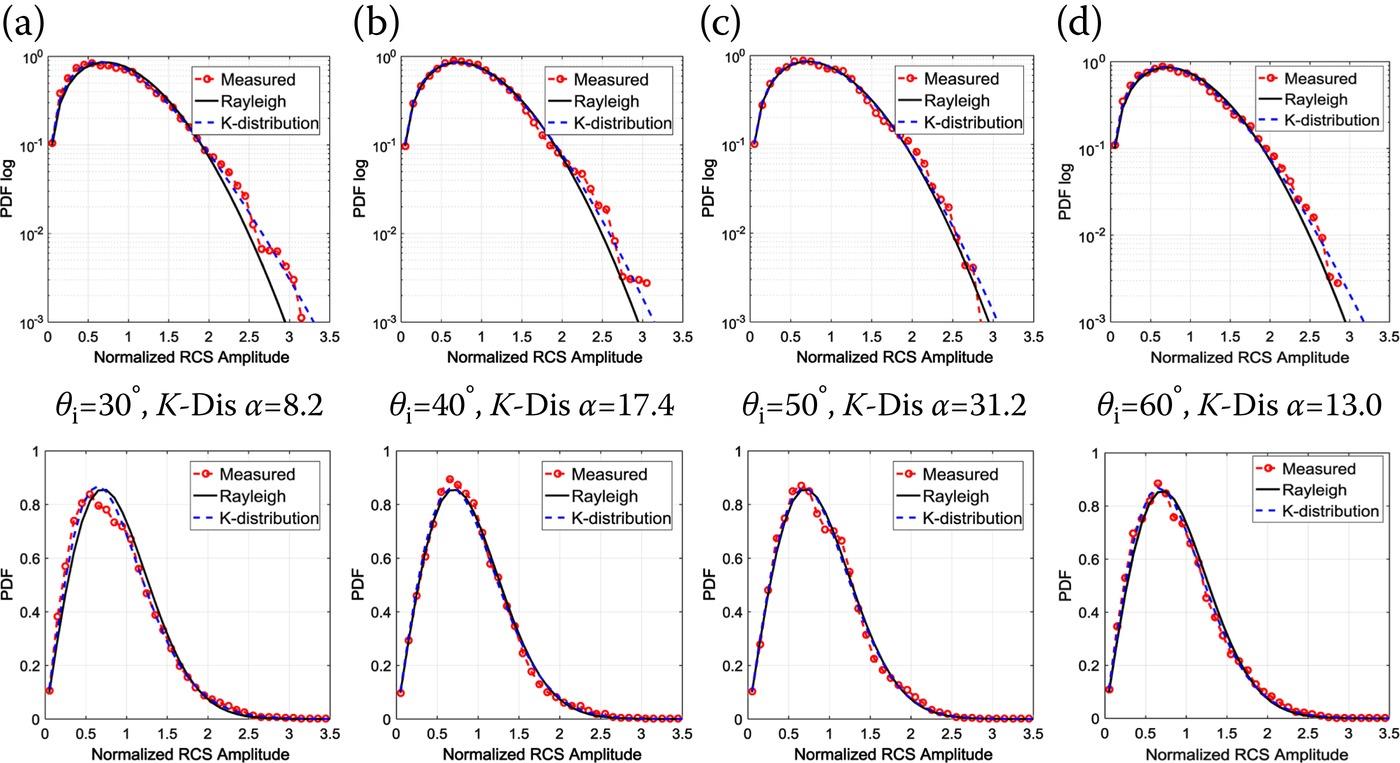
FIGURE 9.10 The normalized amplitude PDF curves of measured images at different , at the resolution cell size of 60 mm, VV, compared with Rayleigh distribution and K-distribution.
After the amplitude PDF results based on experimental images are presented, the corresponding averaged RCS , the averaged scattering coefficients , the fitted α of the K-distribution, and the computed by Equation 6.6 are listed in the Table 9.5 for reference. Further, the computed in case of different are plotted via resolution cell sizes in Figure 9.11. The coarse but not perfect trends can be well observed, that the curves are approaching the theoretical value of with the rising of the resolution cell size. The imperfection in those trends is also due to the limited sample size. Also, in Figure 9.11, the results of computed results without antenna pattern compensation conducted in the imaging process are also presented, showing the necessity of such a treatment in the chamber imaging experiments for speckle properties.
TABLE 9.5
Comparisons of the Average Intensity Values, and Amplitude Speckle Values from the Measured Images at the Resolution Cell Size of 30 and 60 mm
| Resolution | 30° | 40° | 50° | 60° | |
| AIEM (dB) | −6.8 | −8.6 | −10.4 | −11.3 | |
| 30 mm × 30 mm | Average (dBsm) | −37.5 | −39.3 | −41.4 | −43.9 |
| Average (dB) | −6.4 | −7.7 | −9.0 | −10.5 | |
| α for K-dis | 4.5 | 5.2 | 6.3 | 6.0 | |
| Computed | 0.598 | 0.576 | 0.571 | 0.564 | |
| 60 mm × 60 mm | Average (dBsm) | −32.0 | −33.5 | −35.1 | −38.8 |
| Average (dB) | −6.9 | −7.9 | −8.7 | −11.4 | |
| α for K-dis | 8.2 | 17.4 | 31.2 | 13.0 | |
| Computed | 0.562 | 0.532 | 0.534 | 0.555 |
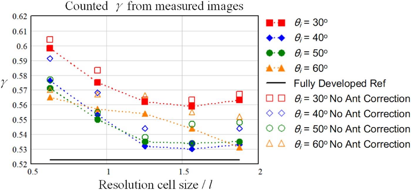
FIGURE 9.11 The computed .. value versus resolution cell size in case of different from the measured images, VV. “No Antenna Correction” denotes for the values from images without the antenna pattern correction procedure.
The simulated scattering coefficients over the upper hemisphere are presented in Figure 9.12, including results by one realization and averaged results by 1600 realizations, for the cases of = 30°, 40°, and 50° of incidence angles. It can be seen that after averaged over 1600 realizations, the computed bistatic scattering coefficients converge to a smooth distribution.
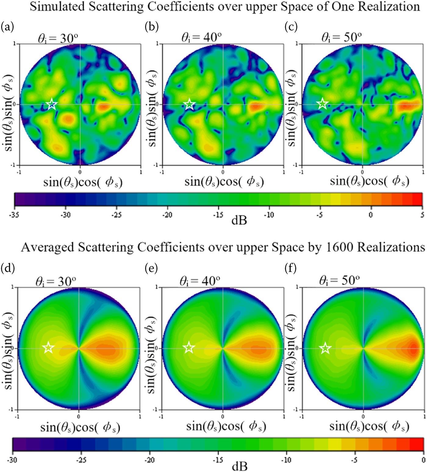
FIGURE 9.12 Results of simulated bistatic scattering coefficients over the upper space, considering different incident angle . The backscattering angular position is marked by the white star symbol.
Then the backscattering amplitude PDF results in cases of , are compared in Figure 9.13, with a 3 dB footprint size of 30 mm in diameter. It is clear that from to , the larger leads to larger fitted a, and the amplitude PDF is more close to the Rayleigh distribution. That trend has also been observed in PDF results from measured images (see Figures 9.9 and 9.10). For reference, the averaged backscattering fitted α for K-distribution, and computed are concluded in Table 9.7. As can be observed from the results in Tables 9.6 and 9.7, both the experimental imaging and numerical simulation statistics show the same trend, that a larger (from 30° to 50°) leads to the closer to the fully developed speckle and thus approaches the theoretical value. That is, as the gets larger in the moderate region, the observed very high-resolution speckle of the exponentially correlated sample approaches the fully developed speckle.
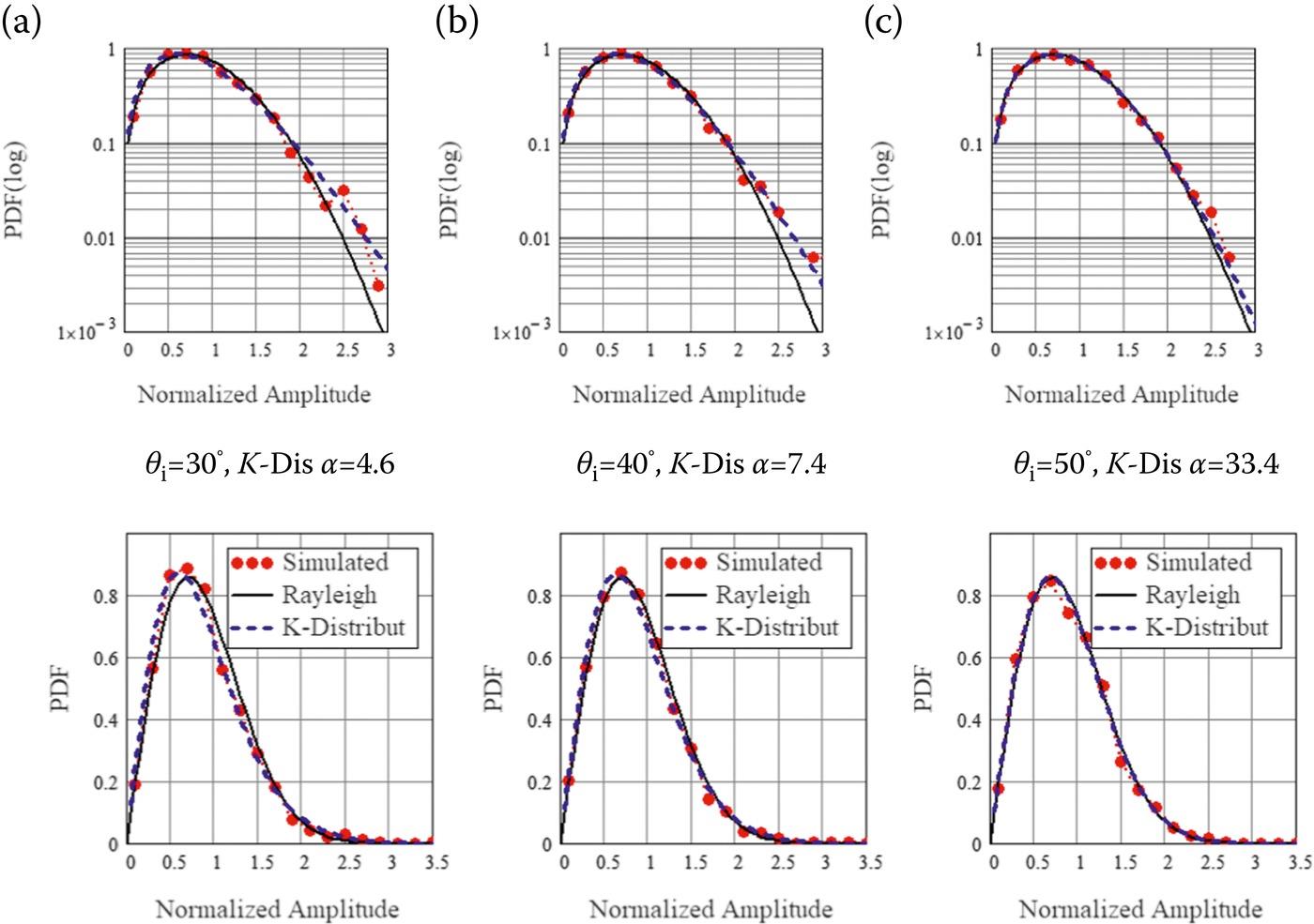
FIGURE 9.13 PDF curves of FDTD-simulated backscattering amplitude at different , at the footprint size of 30 mm, VV, compared with referencing Rayleigh distribution and K-distribution, 1600 realizations.
TABLE 9.7
Comparison of Amplitude in the Case of Imaging Resolution Cell/Footprint Size of 30 mm, at Different , from Measured Images and Simulated Backscattering
| Method \ | 30° | 40° | 50° |
| Imaging Measurement | 0.598 | 0.576 | 0.571 |
| Numerical Simulation | 0.560 | 0.547 | 0.531 |
| Fully Developed speckle | 0.5227 | 0.5227 | 0.5227 |
TABLE 9.6
Comparisons of the Average Intensity Values, and Amplitude Speckle Values from Simulated Backscattering Results by 1600 Realizations, at the Footprint Size of 30 mm
| 30° | 40° | 50° | |
| AIEM (dB) | −6.8 | −8.6 | −10.4 |
| Average (dB) | −7.3 | −9.0 | −10.2 |
| α for K-dis | 4.6 | 7.4 | 33.4 |
| Computed | 0.560 | 0.547 | 0.531 |
It is well known that the high-resolution speckle properties are different from the fully developed speckle that in the case of low-resolution sizes. Driven by the trends of high-resolution imaging system development and deployment, it becomes increasingly desired to model the high-resolution speckle for land observations. Starting from the low-resolution basis, the amplitude PDF of Rayleigh is built on the condition that many independent scatters contribute to one resolution cell. It is straightforward to explore new speckle descriptions based on the concept of an equivalent number of scatterers [9,20].
The K-distribution, especially for the speckle intensity PDF, has been derived based on the mathematical concept of the coherent sum of a finite number of field returns [20]. In that derivation, each of the independent scatters is assumed to be K-distributed in amplitude and uniformly random in phase. Under these assumptions, a close form of K-distribution intensity PDF was obtained. For considering image speckle, the number of scatters per resolution N is an important factor, and it is proportional to α of the overall K-distribution.
The prediction model for the equivalent number of scatterers per resolution cell was proposed in [9] based on the concept of sub-area dividing, to quantitatively predict the speckle properties of rough surfaces in high-resolution observations, and to provide a quantitative description linking the equivalent number of scatterers N to the K-distribution, that a larger N generally leads to speckle closer to Rayleigh and a smaller N may lead to a K-distribution further away from the Rayleigh model. A compact formulation is given as in Equation 9.10, yielding the equivalent number (N) of distributed scatters within a resolution cell size with respect to surface correlation function types, parameters, incident direction, and observation frequency [9]:
where , l is the correlation length; is the area of a resolution cell (not image pixel, and n is 1 for the exponential correlation, 2 for the Gaussian correlation function, with t = 1 [9].
It should be noted that the of the overall K-distribution is also proportional to of the sub-scatters ( ), and a relationship can be concluded as . It is also important that in the rough surface scattering, the namely the K-distribution parameters for the “independent scatter” may vary according to surface roughness parameters and incident angle . It is possible that in the radar image speckle from rough surfaces if there is only one equivalent scatter in a resolution cell, but the scatter is with Gaussian statistics ( is very large), then the overall image speckle properties acts as fully developed. On the other hand, if there is a sufficiently large so that is sufficiently large, then the overall image speckle properties also act nearly as fully developed.
The experimental results demonstrate that larger resolution cell size tends to be more toward Rayleigh distribution, as expected. Physically, when the resolution cell size becomes larger, the equivalent scatterer number gets larger while keep unchanged; therefore, the speckle distribution follows the Rayleigh model. We focus on the scattering from an exponentially correlated rough surface, especially when the resolution is at the level of correlation length. This is a case that will be encountered in the SAR observations of the land surface, as the resolution performance keeps evolving. On the other hand, since the correlation length () of the sea surface is much larger so that the SAR imaging resolution is already at the level of , the non-Rayleigh speckle phenomenon in sea speckle has been widely noticed and studied for decades [10,11,20–23].
Specifically, the K-distribution has also been developed for modeling sea speckles as a compound PDF in [10]. In that derivation, the radar speckle is viewed as a multiplicative process, where the random process y has Rayleigh PDF, with its power modulated by the process x which is assumed to follow the Gamma distribution. The above mathematical description goes along with the physical understanding of a two-scale model for the rough sea surface scattering at intermediate incidence angles [11]. In this case, the backscatter can be regarded as a collection of the small/middle scale returns from the local surfaces such as the Bragg scattering, while the strength of those returns is modulated by the long scale undulation of the surface through tilting and other mechanisms. Apparently, both the scattering from short scale roughness and long scale roughness modulation are functional for the total scattering. Actually, one can find the similarity of the scattering process from exponentially correlated rough surface to that from the sea surface, especially when the resolution cell size is close to the correlation length. In this case, the exponentially correlated rough surface contains rich high-frequency roughness leading to scattering sources all over the surface as the scattering from short-scale roughness, meanwhile, the undulations at the level of correlation length (long scale roughness) provide with the relatively long scale modulation carrier. The difference in the mechanisms between the scattering from an exponentially correlated rough surface observed in high resolution, to that from sea surface, is the lacking of middle scale Bragg scattering. Because on exponentially correlated surface there is no wind-driven periodic undulated structure.
From both the experimental and numerical results at the very high-resolution level, it is interesting to note that when the incident angle gets larger from 30° to 50° (moderate region), the speckle is approaching towards the fully developed Rayleigh description. The answer to this phenomenon, however, can also be found from the knowledge in scattering mechanisms from sea surface [24,25]. In [25], the scattering mechanisms were discussed in the aspects of roughness scales for the two-scale or more precisely multi-scale sea rough surface. Specifically, the wavelength filtering effect states that when the incident angle becomes larger, the dominating factor shifts from the long-scale roughness towards the short-scale roughness [24,25]. And for the vertical polarization, this effect is more notable than that of horizontal polarization [25]. If the effect of long-scale roughness is weakened enough due to the enlarging of in the moderate region, then the multiplicative process is weakened because that the scattering from short-scale is taking the dominance of the scattering mechanism, as well as the speckle properties. And the scattering from short scale roughness most possibly follows a Rayleigh PDF. It is interesting that, from the results of simulated sea backscattering in [22], one can find that the speckle PDF results are also approaching toward Rayleigh when get larger in the moderate region.
From the sea surface scattering, the observed very high-resolution speckle variation from an exponentially correlated rough surface in the moderate region, can be clearly explained: the multiplicative effect of scattering process is weaker when the get larger from small to moderate, as the effects ofcarrier long-scale roughnessgets weaker. In this case, because the scattering from short scale roughness gets more dominating as the get larger and itself acts as Gaussian, the overall speckle distribution approaches towards the Rayleigh model.
The widely applied K-distribution in modeling non-Rayleigh speckle can be either described based on the concepts of equivalent number of (independent) scatter N [9,20] and the two-scale scattering of multiplicative process [10,11]. To further explore the very high-resolution speckle properties from exponentially correlated rough surface as a significant description for ground roughness, and to discuss the dominating factors, another set of computations are performed for analysis. Specifically, different RMS heights are considered: 2 mm (0.21λ), 4 mm (0.43λ), 8 mm (0.85λ), 12 mm (1.28λ@32 GHz) at . For each RMS height , a total of 1600 realizations are computed for the speckle analysis. In Figure 9.14, the electric fields at 32 GHz in the incident plane cut of the computation domain in one specific realization were presented, as an intuitive exhibition for the difference of scattering process in case of different RMS heights. It seems that when σ = 4 mm, occasional specular reflection may contribute to the backscattering of . As shown in the scattering coefficient results of Figure 9.15, the backscattering at σ = 4 mm is larger than those at σ = 2 mm, σ = 8 mm, and σ = 12 mm. In Figure 9.15, it is also interesting to observe that as the σ changes from 2 to 12 mm, the dominant bistatic scattering region gradually moves from the forward region (σ = 2 mm) to the backward region (σ = 12 mm). Also, the averaged computed backscattering coefficients are listed in Table 9.5, and a good agreement with the AIEM results can be observed.
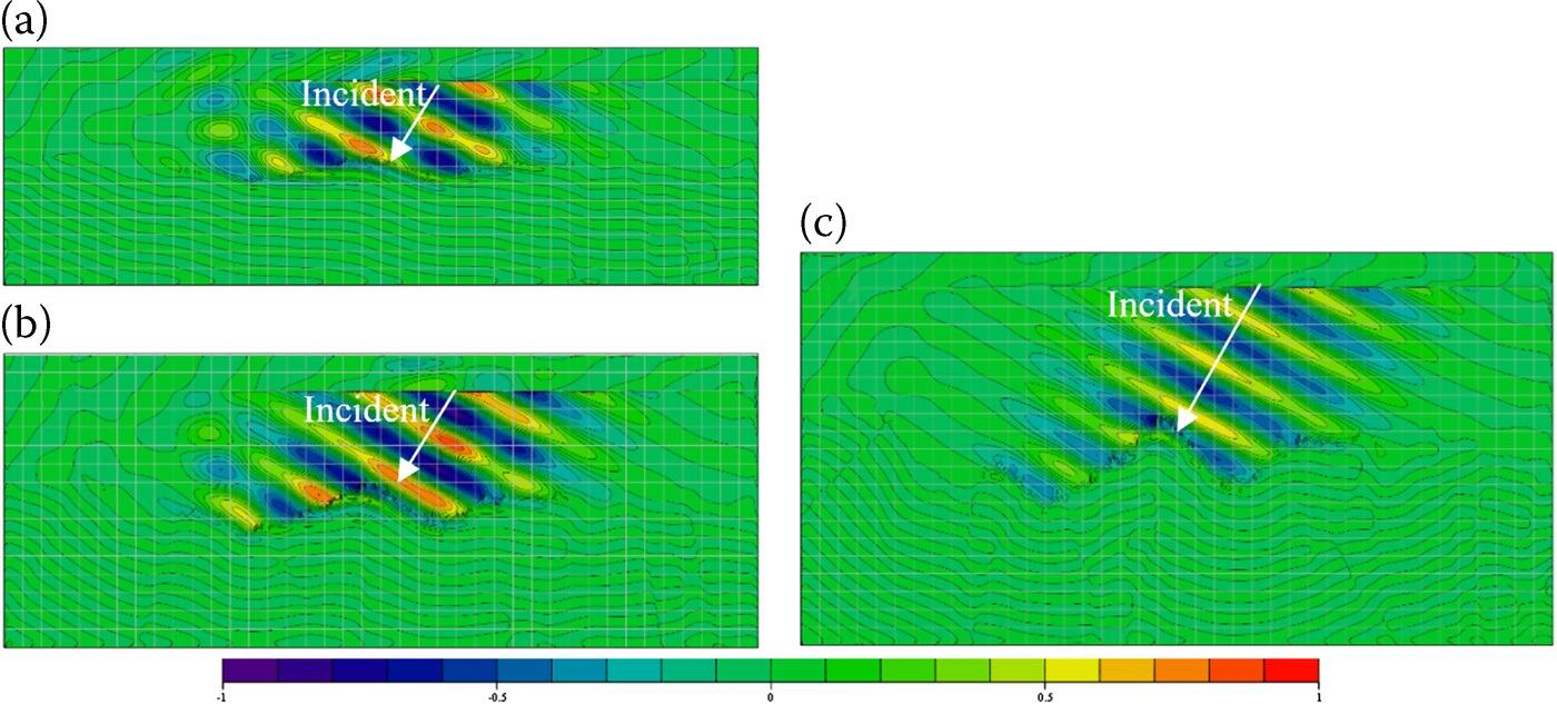
FIGURE 9.14 Recorded total field (E-Field, maximum normalized, real part) in the incident plane cut from the exponentially correlated rough surface simulation, . (a) σ = 2 mm, (b) σ = 4 mm, (c) σ = 8 mm.
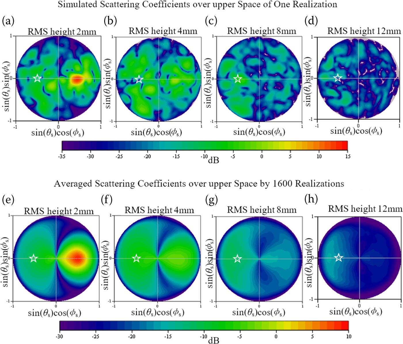
FIGURE 9.15 Results of simulated bistatic scattering coefficients over the upper space, considering different RMS height (σ). The backscattering location is marked by the white star symbol.
The computed amplitude speckle results are then presented in Figure 9.16 and Table 9.8, showing that: at the lowest and highest considered RMS height values, the backscattering speckle amplitude PDF is very close to the Rayleigh distribution; meanwhile at the moderate σ of 4 mm, the PDF is away from the Rayleigh one. The observed trends of speckle properties are interesting that it can be directly explained by neither the concept of an equivalent number of scatterers (see Equation 9.10), nor two-scale scattering multiplicative process as the scattering scale factor. The equivalent number of scatterers theory predicts that the N varies from several, to tens and then to thousands, as the RMS height changes from 2 mm to 12 mm, at the resolution level of 30 mm and . Keeping in mind that the overall α is proportional to both the N and the statistical property of each independent scatters ( ), in the theoretic framework of an equivalent number of scatterers αe (N*αs) is the statistical property of an equivalent number of scatterers, and αs is assumed to be 0.1. The rapid change of the estimated αs shown in the last line of Table 9.8 as the RMS heights vary from 2 mm to 4 mm, is hard to predict when using the equivalent number of scatters theory if one does not consider full scattering mechanisms. It is understood that when the RMS height increases, the long scale undulation is stronger, and thus the two-scale multiplicative scattering process is enhanced. However, it is not clear how the counted α keeps gets larger as the RMS height increases from 4 mm to 12 mm (Table 9.8), simply from a two-scale multiplicative scattering process. Actually, it is most likely that both of the two effects should be considered in analyzing and modeling the very high-resolution speckle from exponentially correlated rough surface.
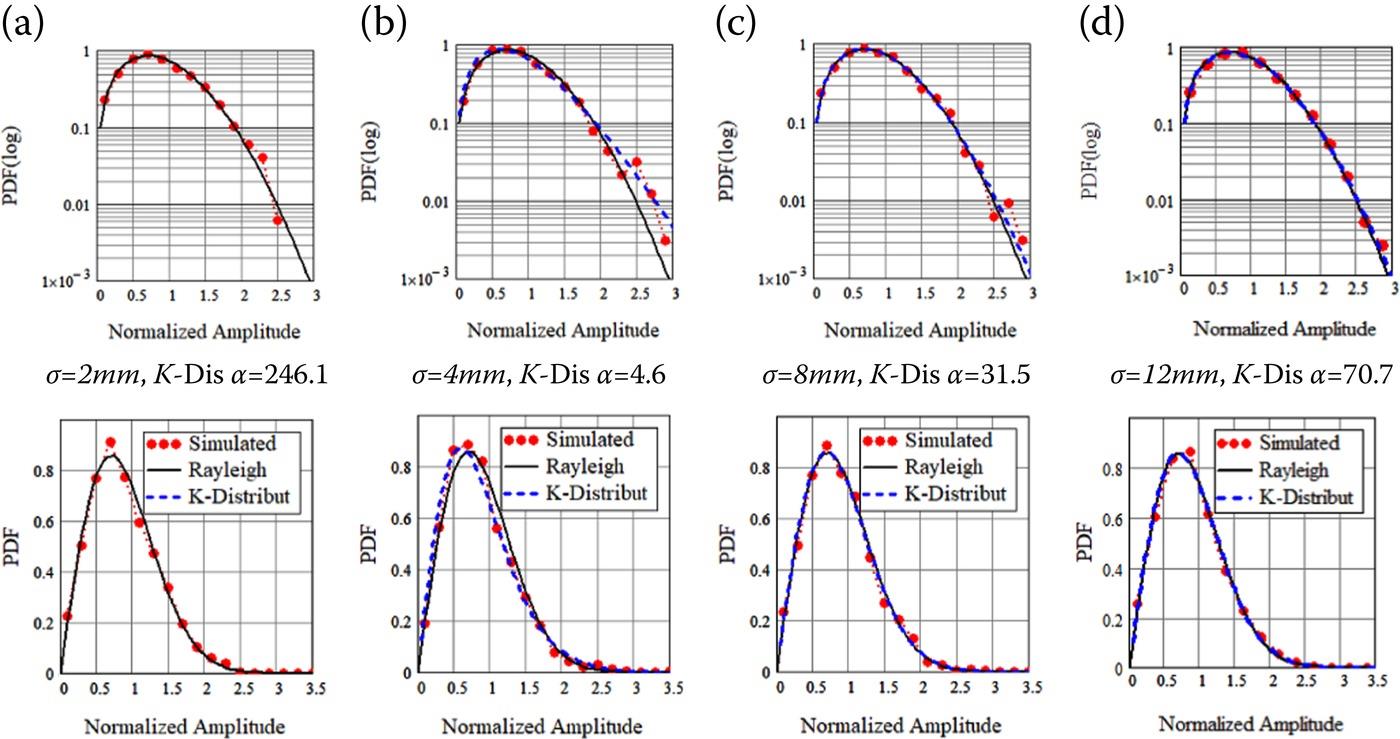
FIGURE 9.16 PDF curves of FDTD-simulated backscattering amplitude at , considering exponentially correlated surface with different RMS heights , (a): σ = 2 mm; (b): σ = 4 mm; (c): σ = 8 mm; (d): σ = 12 mm. VV, compared with referencing Rayleigh distribution and K-distribution, 1600 realizations. (a) σ = 2 mm, K-Dis α = 246.1 (b) σ = 4 mm, K-Dis α = 4.6 (c) σ = 8 mm, K-Dis α = 31.5 (d) σ = 12 mm, K-Dis α = 70.7.
TABLE 9.8
Comparisons of the Average Intensity Values, and Amplitude Speckle Values from Simulated Backscattering Results by 1600 Realizations, at the Footprint Size of 30 mm (3.2λ, 0.63l )
| RMS Height σ | 2 mm | 4 mm | 8 mm | 12 mm |
| AIEM (dB) | −10.4 | −6.8 | −11.8 | −18.2 |
| Numerical (dB) | −10.0 | −7.3 | −12.0 | −17.7 |
| Amplitude | 0.525 | 0.56 | 0.535 | 0.528 |
| for K-dis | 246.1 | 4.6 | 31.5 | 70.7 |
| ENS Prediction | 2.4 | 43.4 | 719.9 | 3668 |
| ENS Predicted αe | 0.24 | 4.34 | 72.0 | 366.8 |
| 102.5 | 0.106 | 0.04 | 0.019 |
When the RMS height is 2 mm, the slope of the rough surface is very small (0.042). Although the predicted equivalent number of scatterers within resolution cell size is small, those short-scale scatters remain a random Gaussian process without notable long-scale modulation. Therefore, with a large number of realizations (or return cells) the speckle remains the fully developed Rayleigh description. When the RMS height is 12mm, the slope of the rough surface gets to 0.25, the process of long scale modulation of scattering from short-scale roughness should be notable. However, the equivalent scatterer number is too large (thousands) in this case, it is very likely that such a large amount of scatters overwhelms the modulation effect, so that the very high-resolution speckle is close to the fully developed speckle again. It is worthy to look back to the case of σ = 4 mm. One can find that in this case, the scatterer number is moderate (tens) and not large enough; then the notable two-scale modulation effect drives the speckle PDF away from the Rayleigh distribution to the K-distribution with a moderate α.
From the above discussions on the very high-resolution speckle properties from exponentially correlated rough surfaces representing ground roughness by means of experimental measurements and numerical simulations, we can summarize that both the equivalent scatterer number theory and scattering scale description of two-scale multiplicative process is informative and perspective in analyzing the experimental and numerical results of very high-resolution SAR images. However, by neither of them one can comprehensively explain the observed trends in the results. It is evident from the results that if the equivalent number of scatterers is not sufficiently large, the two-scale multiplicative scattering process may drive the VHR speckle PDF away from the fully developed Rayleigh description. Also, the dominance of the sufficient large equivalent number of scatterers is also observed, and that leads the VHR speckle properties close to the fully developed model even when the resolution cell size is smaller than the correlation length. It is confirmed that the equivalent number of scatterers may be useful in setting a bar for the very high-resolution speckle modeling on exponentially correlated rough surfaces, below which the multiplicative scattering process should be considered, and above that bar the Rayleigh model can be sufficient for modeling speckles.
References
1. Chen, K. S., Tsang, L., Chen, K. L., Liao, T. H., and Lee, J. S., Polarimetric simulations of SAR at L-Band over bare soil using scattering matrices of random rough surfaces from numerical three-dimensional solutions of Maxwell equations, IEEE Transactions on Geosciences and Remote Sensing, 52(11), 7048–7058, 2014.
2. Ulaby, F. T., Moore, R. K., and Fung, A. K., Microwave Remote Sensing: Active and Passive, Addison-Wesley, Reading, MA, 1981.
3. Tsang, L., Kong, J. A., and Ding, K. H., Scattering of Electromagnetic Waves: Theories and Applications, John Wiley & Sons, New York, 2000.
4. Lee, J. S., and Pottier, E., Polarimetric Radar Imaging: From Basics to Applications, CRC Press: Boca Raton, FL, 2009.
5. Sarabandi, K., and Oh, Y., Effect of antenna footprint on the statistics of radar backscattering from random surfaces. In Proceedings of the IEEE IGARSS, Firenze, Italy, 10–14, pp. 927–929, July 1995.
6. Allain, S., Ferro-Famil, L., Pottier, E., and Fortuny, J., Influence of resolution cell size for surface parameter retrieval from polarimetric SAR data. Proceedings of the IEEE IGARSS, Toulouse, France, 21–25, pp. 440–442, July 2003.
7. Park, S. E., Ferro-Famil, L., Allain, S., and Pottier, E., Surface roughness and microwave surface scattering of high-resolution imaging radar, IEEE Geoscience and Remote Sensing Letters, 12(4), 756–760, 2015.
8. Nesti, G., Fortuny, J., and Sieber, A. J., Comparison of backscattered signal statistics as derived from indoor scatterometric and SAR experiments. IEEE Transactions on Geoscience and Remote Sensing, 34(5), 1074–1083, 1996.
9. Di Martino, G., Iodice, A., Riccio, D., and Ruello, G., Equivalent number of scatterers for SAR speckle modeling, IEEE Transactions on Geoscience and Remote Sensing, 52(51), 2555–2564, 2014.
10. Ward, K. D., Tough, R. J. A., Watts, S., Sea Clutter: Scattering, the K Distribution and Radar Performance, IET, London, UK, 2006.
11. Valenzuela, G. R., Theories for the interaction of electromagnetic and oceanic waves—A review. Boudary-Layer Meteorology, 13, 61–85, 1978.
12. Whitt, M. W., Ulaby, F. T., Polatin, P., and Liepa, V. V., A general polarimetric radar calibration technique, IEEE Transactions on Antennas and Propagation, 39(1), 62–67, 1991.
13. Freeman, A., Van Zyl, J. J., Klein, J. D., Zebker, H. A., and Shen, Y., Calibration of Stokes and scattering matrix format polarimetric SAR data, IEEE Transactions on Geoscience and Remote Sensing, 30(3), 531–539, May 1992.
14. Van Zyl, J. J., Calibration of polarimetric radar images using only image parameters and trihedral corner reflector responses, IEEE Transactions on Geoscience and Remote Sensing, 28(3), 337–348, May 1990.
15. Sarabandi, K., Ulaby, F. T., and Dobson, M. C., AIRSAR and POLARSCAT cross-calibration using point and distributed targets, IEEE Transactions on Geoscience and Remote Sensing, 2(4), 18–21, August 1993.
16. Touzi, R., and Shimada, M., Polarimetric PALSAR calibration, IEEE Transactions on Geoscience and Remote Sensing, 47(12), 3951–3959, December 2009.
17. Rabus, B., Wehn, H., and Nolan, M. The importance of soil moisture and soil structure for insar phase and backscatter, as determined by FDTD modeling, IEEE Transactions on Geoscience and Remote Sensing, 48(5), 2421–2429, 2010.
18. Giannakis, I., Giannopoulos, A., and Warren, C., A realistic FDTD numerical modeling framework of ground penetrating radar for landmine detection, IEEE Journal of Selected Topics in Applied Earth Observervations and Remote Sensing, 9(1), 37–51, 2016.
19. Bai, M., Jin, M., Ou, N., and Miao, J., On scattering from an array of absorptive material coated cones by the PWS approach, IEEE Transactions on Antennas Propagation, 61(6), 3216–3224, 2013.
20. Jakeman, E., and Pusey, P. N., A model for non-Rayleigh sea echo, IEEE Transactions on Antennas Propagation, 24(6), 806–814, 1976.
21. Nouguier, F., Guérin, C.-A., and Chapron, B., Scattering from nonlinear gravity waves: The ‘Choppy Wave’ model, IEEE Transactions on Geoscience and Remote Sensing, 48(12), 4184–4192, 2010.
22. Pinel, N., Chapron, B., Bourlier, C., de Beaucoudrey, N., Garello, R., and Ghaleb, A., Statistical analysis of real aperture radar field backscattered from sea surfaces under moderate winds by Monte Carlo simulations, IEEE Transactions on Geoscience and Remote Sensing, 52(1), 6459–6470, 2014.
23. Durden, S. L., and Vesecky, J. F., A physical radar cross-section model for a wind-driven sea with swell. IEEE Journal of Oceanic Engineering, 10(4), 445–451, 1985.
24. Durden, S. L. and Vesecky, J. F., A numerical study of the separation wavenumber in the two-scale scattering approximation (ocean surface radar backscatter). IEEE Transactions on Geoscience and Remote Sensing, 28(2), 271–272, 1990.
25. Fung, A. K., Backscattering from Multiscale Rough Surfaces with Application to Wind Scatterometry, Artech House, Norwood, MA, 2015.