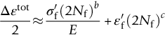
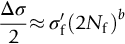
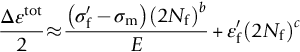
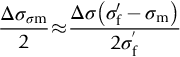
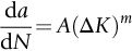
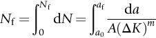
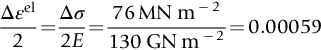
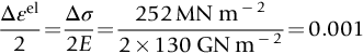
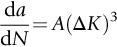
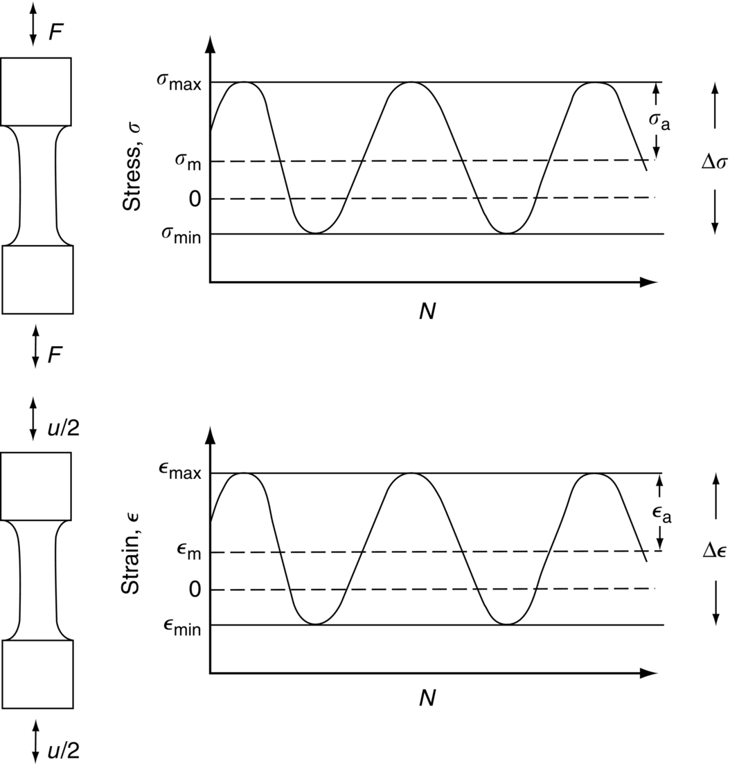
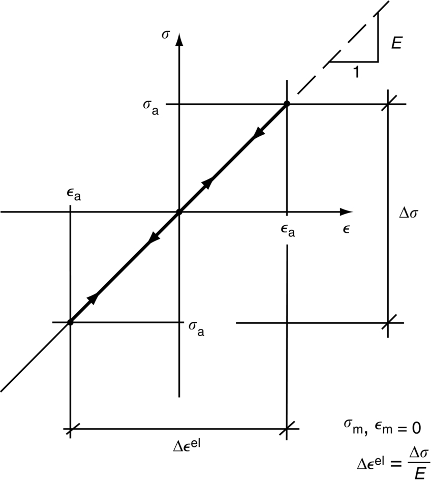
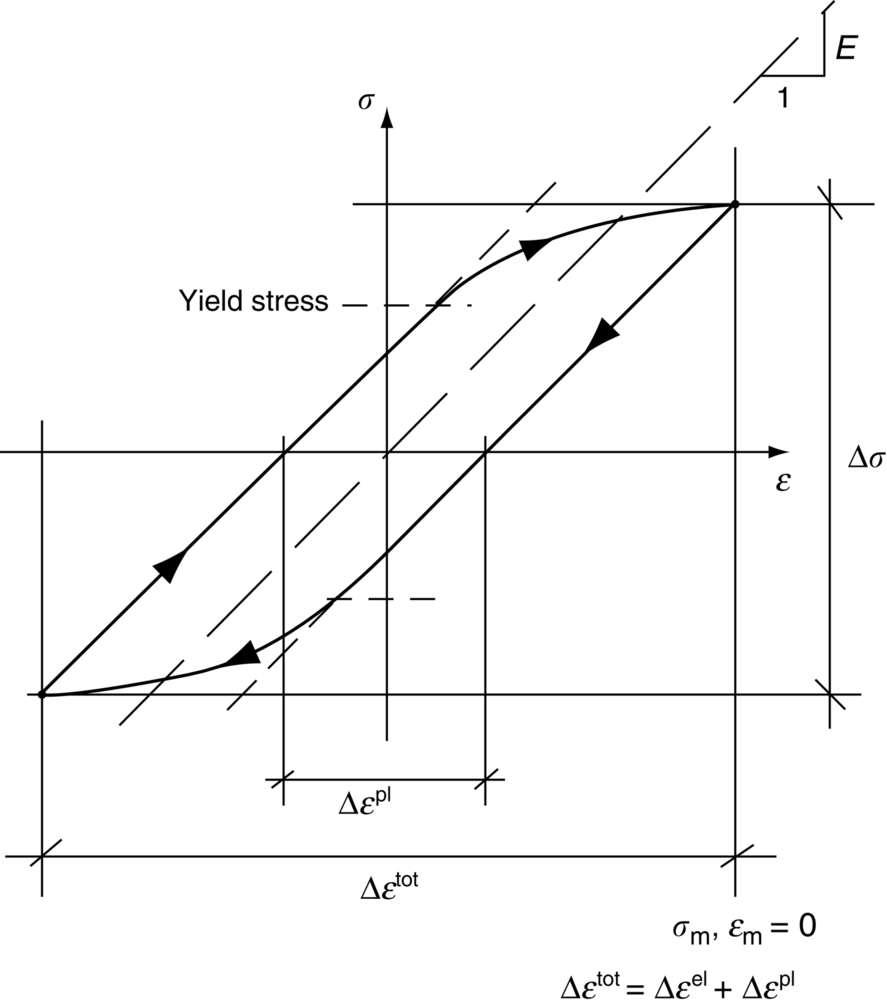
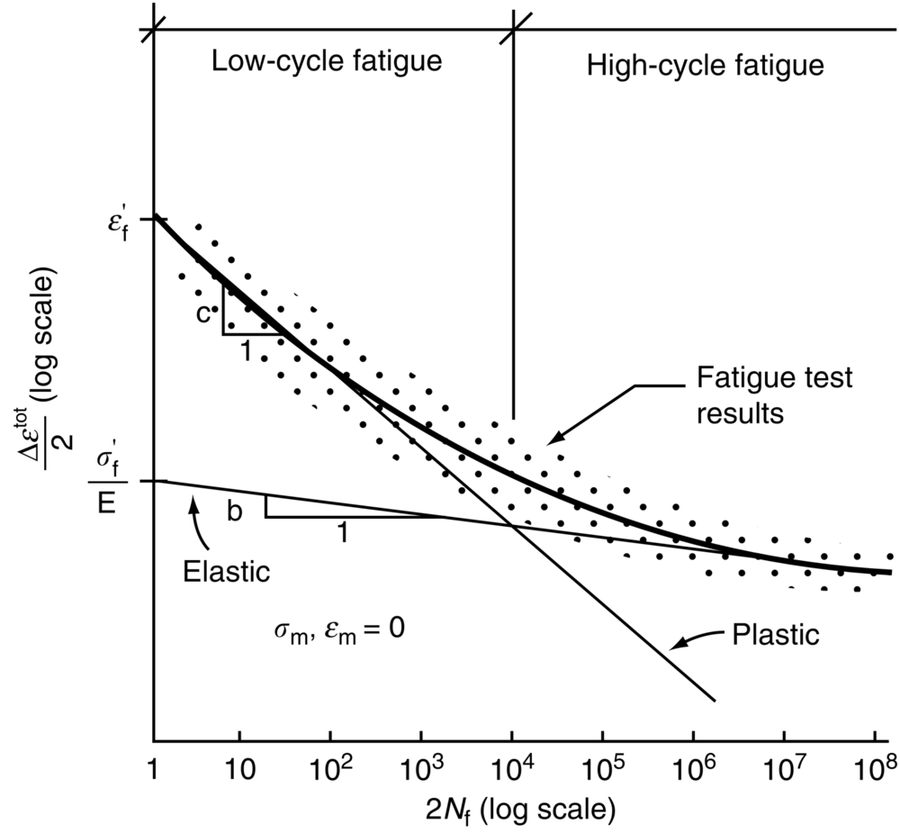
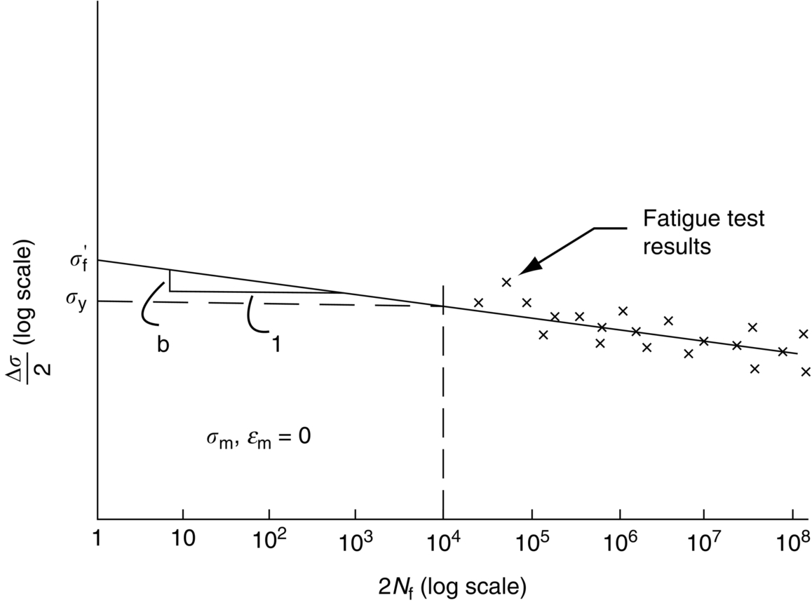
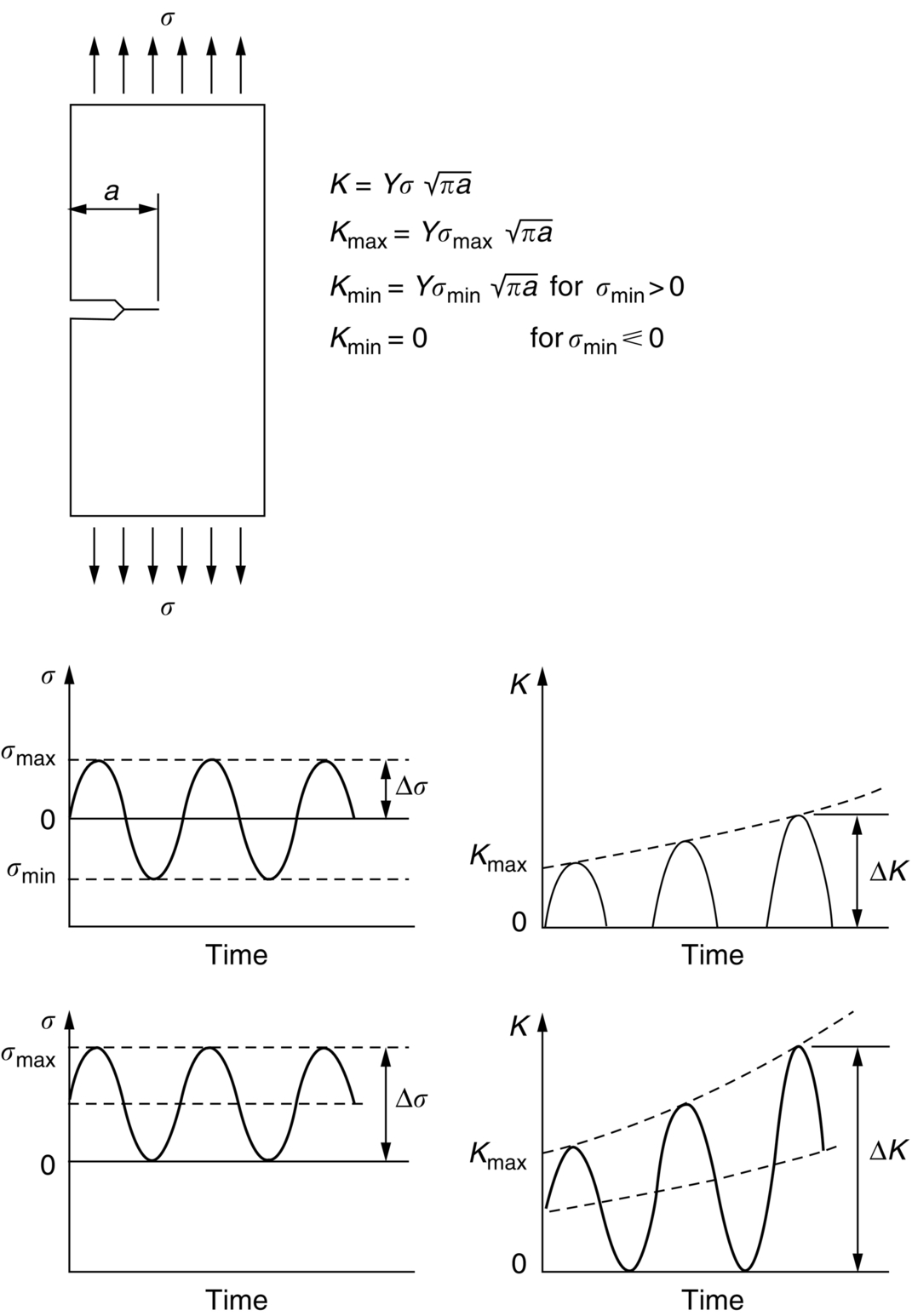
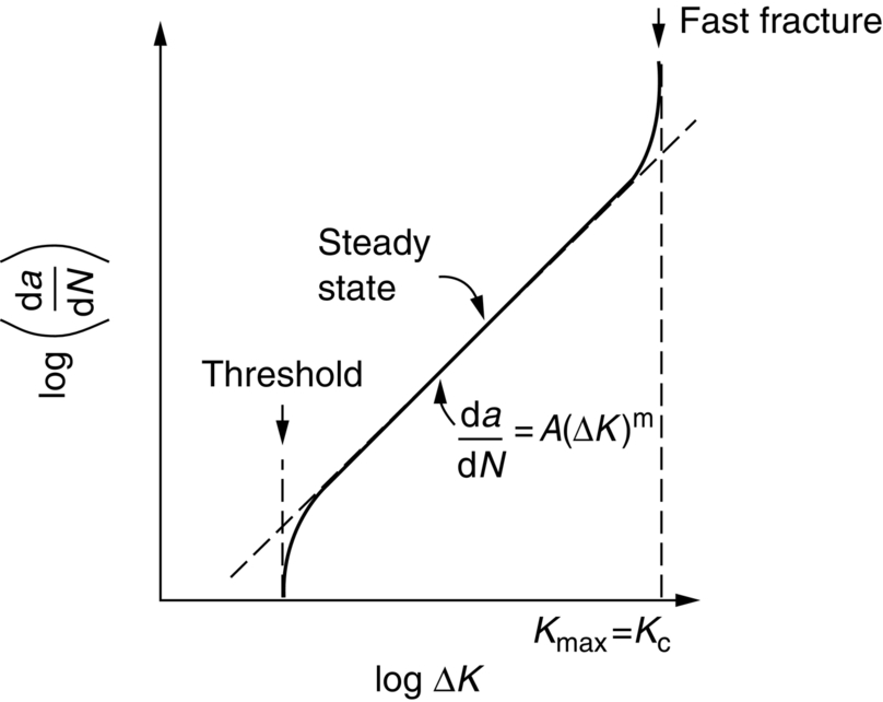
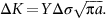
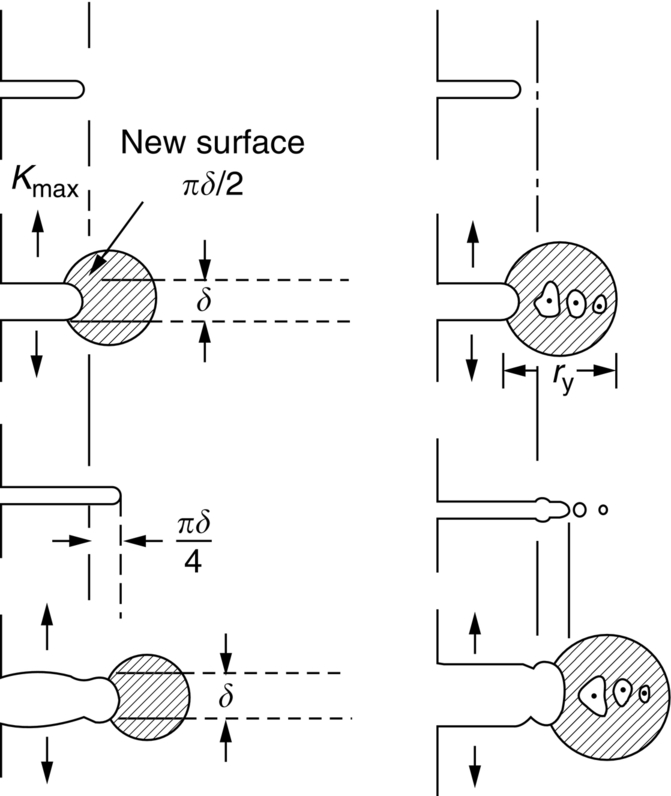
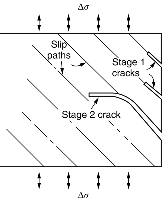
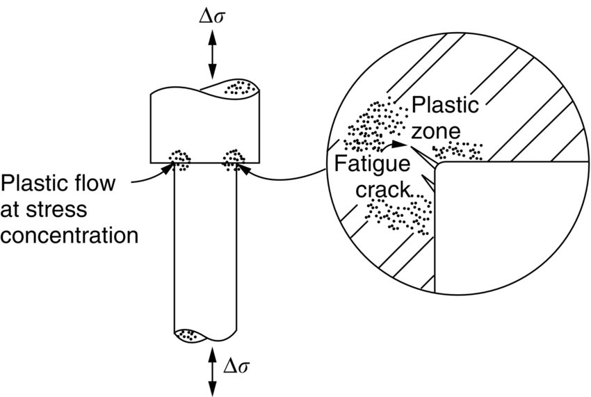
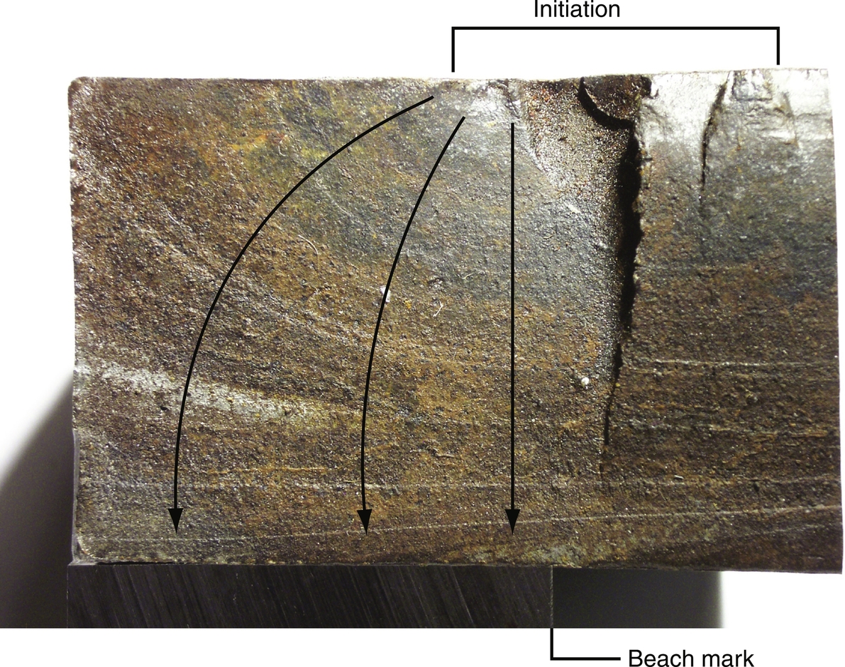
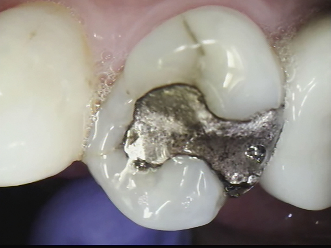
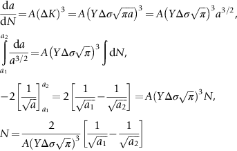
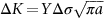
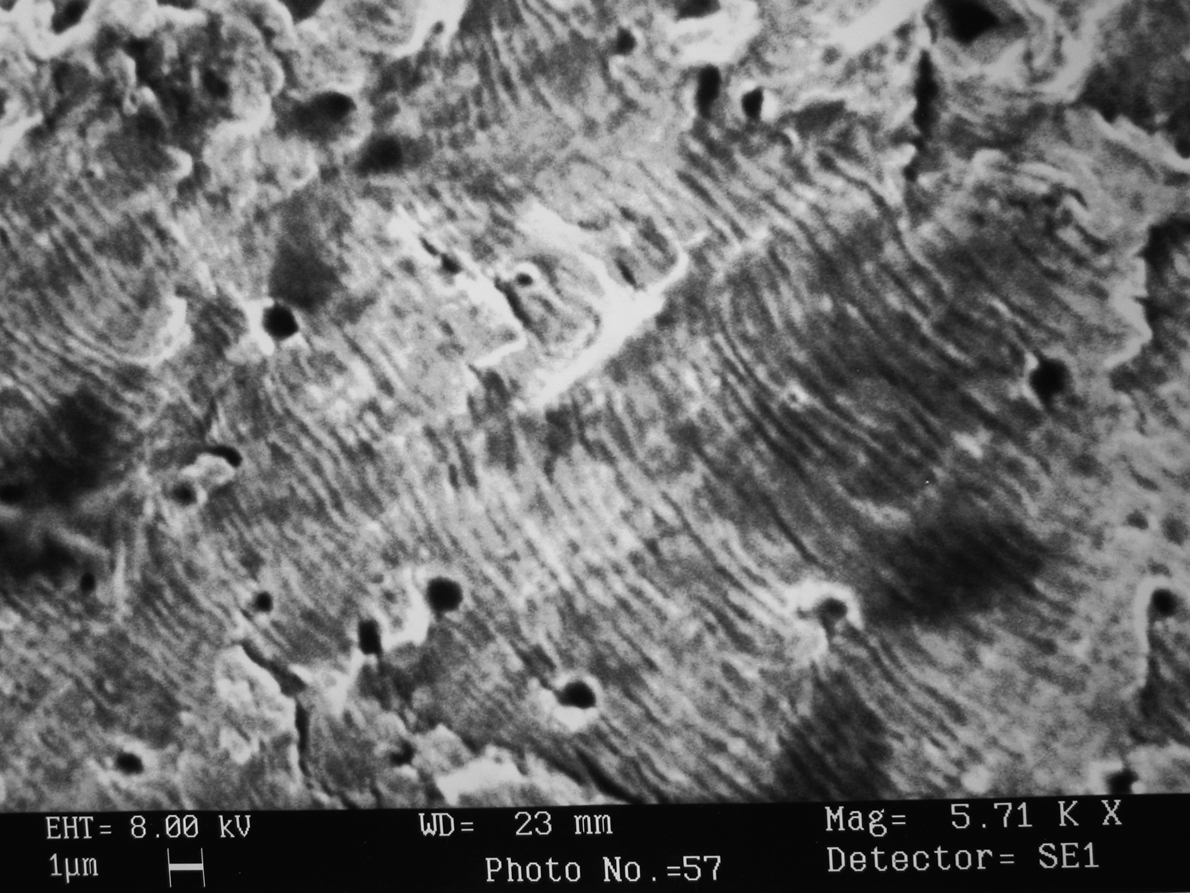
section epub:type=”chapter”> This chapter examines the condition under which a crack is stable and would not grow, as is the condition under which it would propagate catastrophically by fast fracture. If the maximum size of crack in the structure is known, then a working load at which fast fracture will not occur can be chosen. But cracks can form, and grow slowly, at loads lower than this, if the load is cycled. The process of slow crack growth—fatigue—is the subject of this chapter. Fatigue tests are done by subjecting specimens of the material to a cyclically varying load or displacement. For simplicity, the time variation of stress and strain is shown as a sine wave, but modern testing machines are capable of applying almost any chosen load or displacement spectrum. The chapter discusses fatigue of uncracked components and that of cracked components. This chapter concludes with a discussion of various fatigue mechanisms. In Chapters 14 and 15, we examined the conditions under which a crack was stable, and would not grow, and the condition under which it would propagate catastrophically by fast fracture. If we know the maximum size of crack in the structure we can then choose a working load at which fast fracture will not occur. But cracks can form, and grow slowly, at loads lower than this, if the load is cycled. The process of slow crack growth—fatigue—is the subject of this chapter. When the clip of your pen breaks, when the pedals fall off your bicycle, when the handle of the refrigerator comes away in your hand, it is usually fatigue which is responsible. Fatigue tests are done by subjecting specimens of the material to a cyclically varying load or displacement (Figure 18.1). For simplicity, the time variation of stress and strain is shown as a sine wave, but modern testing machines are capable of applying almost any chosen load or displacement spectrum. The specimens are subjected to increasing numbers of fatigue cycles N, until they finally crack (when N = Nf—the number of cycles to failure). Figure 18.2 shows how the cyclic stress and cyclic strain are coupled in a linear elastic specimen. The stress and strain are linearly related through Young’s modulus, and the stress range Δσ produces (or is produced by) an elastic strain range Δɛel (equal to Δσ/E). Figure 18.3 shows how the cyclic stress and cyclic strain are coupled in a specimen that is cycled outside the elastic limit. There is no longer a simple relationship between stress and strain. Instead, they are related by a stress–strain loop, which must be determined from tests on the material. In addition, the shape of the loop changes with the number of cycles, and it can take several hundred (or even thousand) cycles before the shape of the loop stabilizes. The stress range Δσ produces (or is produced by) a total strain range Δɛtot—which is the sum of the elastic strain range Δɛel and the plastic strain range Δɛpl. The best way to correlate fatigue test data is on a log-log plot of the total strain amplitude Δɛtot/2 versus the number of reversals to failure 2Nf (there are two reversals of load or displacement in each complete cycle). Figure 18.4 shows the shape of the curve on which the data points typically fall (although there is usually a lot of experimental scatter on either side of the curve). It is useful to know that this curve is the sum of two linear relationships on the log–log plot: (a) between the elastic strain amplitude and 2Nf, and (b) between the plastic strain amplitude and 2Nf. It can be approximated mathematically as: b and c are constants determined by fitting the test data—they are generally in the range –0.05 to –0.12 for b, and –0.5 to –0.7 for c. The data in Figure 18.4 can be divided into two régimes: Until the 1950s, most fatigue studies were concerned with high-cycle fatigue (HCF), since engineering components subjected to cyclic loadings (e.g., railway axles, engine crankshafts, bicycle frames) were designed to keep the maximum stress below the elastic limit. Because of this, it is still common practice to plot HCF data on a log–log plot of the stress amplitude Δσ/2 versus 2Nf—see Figure 18.5. The test data can then be approximated as: So far, we have only considered test data obtained with zero mean stress (σm = 0). However, in many design situations, there will be a tensile mean stress (σm > 0). Intuitively, we would expect that the component would be more prone to fatigue if it were subjected to a large mean stress in addition to having to cope with repeated cycles of stress. The test data confirm this—to keep the fatigue life the same when the mean stress is increased from 0 to some large tensile value, the stress (or strain) cycles must be reduced in amplitude to compensate. In terms of the strain approach to fatigue, the test data can be approximated as follows: The equation clearly shows that, to keep the fatigue life the same, the strain amplitude must be decreased to compensate for a mean stress. In terms of the stress approach to fatigue, the test data can be approximated as: Δσ/2 is the stress amplitude for failure after a given number of cycles with zero mean stress, and Δσσm/2 is the stress amplitude for failure after the same number of cycles but with a mean stress. So if, for example, the mean stress is half the fracture stress, then the applied stress amplitude must be halved to keep the fatigue life the same. Large structures—particularly welded structures such as bridges, ships, oil rigs, and nuclear pressure vessels—always contain cracks. All we can be sure of is that the initial length of these cracks is less than a given length—the length we can reasonably detect when we check or examine the structure. To assess the safe life of the structure we need to know how long (for how many cycles) the structure can last before one of these cracks grows to a length at which it propagates catastrophically. Data on fatigue crack propagation are gathered by cyclically loading specimens containing a sharp crack like that shown in Figure 18.6. We define The cyclic stress intensity ΔK increases with time (at constant load) because the crack grows in tension. It is found that the crack growth per cycle, da/dN, increases with ΔK in the way shown in Figure 18.7. In the steady-state régime, the crack-growth rate is described by where A and m are material constants. Obviously, if a0 (the initial crack length) is given, and the final crack length (af) at which the crack becomes unstable and runs rapidly is known or can be calculated, then the safe number of cycles can be estimated by integrating the equation remembering that Cracks grow in the way shown in Figure 18.8. In a pure metal or polymer (left diagram), the tensile stress produces a plastic zone (Chapter 15) which makes the crack tip stretch open by the amount δ, creating new surface there. As the stress is removed the crack closes and the new surface folds forward extending the crack (roughly by δ). On the next cycle the same thing happens again, and the crack inches forward, roughly at da/dN ≈ δ. Note that the crack cannot grow when the stress is compressive because the crack faces come into contact and carry the load (crack closure). We mentioned in Chapter 15 that real engineering alloys always have little inclusions in them. Then (see right diagram of Figure 18.8), within the plastic zone, holes form and link with each other, and with the crack tip. The crack now advances a little faster than before, aided by the holes. In precracked structures these processes determine the fatigue life. In uncracked components subject to low-cycle fatigue, the general plasticity quickly roughens the surface, and a crack forms there, propagating first along a slip path (“Stage 1” crack) and then, by the mechanism we have described, normal to the tensile axis (Figure 18.9). High-cycle fatigue is different. When the stress is below general yield, almost all of the life is taken up in initiating a crack. Although there is no general plasticity, there is local plasticity wherever a notch or scratch or change of section concentrates stress. A crack ultimately initiates in the zone of one of these stress concentrations (Figure 18.10) and propagates, slowly at first, and then faster, until the component fails. For this reason, sudden changes of section or scratches are very dangerous in high-cycle fatigue, often reducing the fatigue life by orders of magnitude. Figure 18.11 shows the crack surface of a steel plate (40 mm thick) which failed by fatigue. The shape of the fatigue crack at any given time is indicated by “beach marks”. Figure 18.12 shows a fatigue crack in a human tooth caused by the repeated loads of chewing food. You have just been told that some copper water-cooling plates have begun failing in a furnace. The suspected cause is low-cycle fatigue, caused by thermal expansion movements between the cooling plates and the furnace shell. To make a preliminary assessment, you urgently need the strain–life plot for annealed deoxidized copper—the material of the plates. But where do you start? Remember that Figure 18.4 shows the typical form of the strain–life plot. Looking at the left side of the plot, you can see that it should at least be possible to find standard tensile testing data for copper, which would give you values for the true fracture stress and strain. There are plenty of handbooks and/or websites that can give you tensile test data, but of course this is always listed as nominal stress and strain, so needs to be converted into true stress and strain. This is OK, because you already know about the equations that do this conversion (see Chapter 9). You also need a value for Young’s modulus, but again that is easily available (and will be the same whatever the grade of copper). You easily locate the necessary data for annealed copper: σTS = 216 MN m-2, ɛf = 48% → 0.48, E = 130 GN m-2. Then: So you already have two critical points to put on your plot—we have marked them on the diagram. We could now do with something at the right side of the plot, to define the elastic fatigue line. There are lots of data available for HCF—in fact, much more than there are for LCF. But almost always, handbooks and/or websites list just one value—the stress amplitude for failure after typically 108 cycles. In the case of annealed copper, a quick handbook search comes up with a stress of ±76 MN m-2 after 2 × 10⁷ cycles (4 × 10⁷) reversals. The strain amplitude corresponding to the stress amplitude of 76 MN m-2 is: Marking this point on the diagram fixes the elastic fatigue line. Finally, we need some points in the middle of the plot, to define the plastic line. Then we can just add the plastic line and the elastic line to get the overall strain–life plot (but remember that the vertical axis is not a linear scale!). Fortunately, a quick trawl through some standard textbooks comes up with a drawing of the cyclic stress–strain loop for annealed copper under a fixed strain range of 0.0084 (Hertzberg). The stabilized stress range is 252 MN m-2, and the number of reversals to failure is 8060. The total strain amplitude is then 0.0042. The elastic part of the total strain amplitude is: The plastic part of the total strain amplitude is then 0.0042 − 0.001 = 0.0032. The three strain amplitudes are marked on the preceding diagram, and they allow the overall strain–life plot to be drawn. This is sufficient for your preliminary assessment. However, predictive design should always rely on actual fatigue test data—and plenty of it, so that the variability of the data (mean and standard deviation) can be established. In Equation (18.5), we showed that the rate of fatigue crack growth was proportional to (ΔK)m, where ΔK is the range of the stress intensity for the crack, and m is a material constant. In Equation (18.6), we showed that we could calculate the number of fatigue cycles Nf required to grow the crack from an initial length to a final length by integrating up Equation (18.5). The integration is somewhat tricky, so we give an example of it here, using a value of m = 3 (which is typical for steels). Starting with an Equation of the kind (18.5), we get Typically, A = 6 × 10–12 m (MN m–3/2)–3. We assume Y = 1, and Δσ = 100 MN m–2. We assume initial and final cracks of length 2 mm and 10 mm. To get the units right, these must be converted into m, i.e., to 0.002 m and 0.010 m. We then input numbers as follows Putting the units in verifies that N is dimensionless, as it must be. Next time, there is no need to write out the units as long as they are all in MN and m. about a mean tensile stress of Δσ/2. Given that
Fatigue Failure
Publisher Summary
18.1 Introduction
18.2 Fatigue of Uncracked Components
 and
and  are the true fracture stress and true fracture strain (derived from a standard tensile test on the material).
18.3 Fatigue of Cracked Components
18.4 Fatigue Mechanisms
Worked Example 1
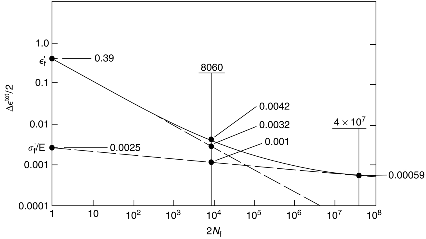
Worked example 2

Examples
Rating of appliance
1.2 kW
Power supply
250 V, 50 Hz AC
Fuse rating of plug
13 A
Flex
3 conductors (live, neutral, and earth) each rated 13 A
Individual conductor
23 strands of copper wire in a polymer sheath; each strand 0.18 mm in diameter
Age of iron
14 years
Estimated number of movements of iron
106
where A = 6 × 10-12 m (MN m-3/2)-3. The component is subjected to an alternating stress of range
 , estimate the number of cycles to failure. Assume that Y = 1.12.
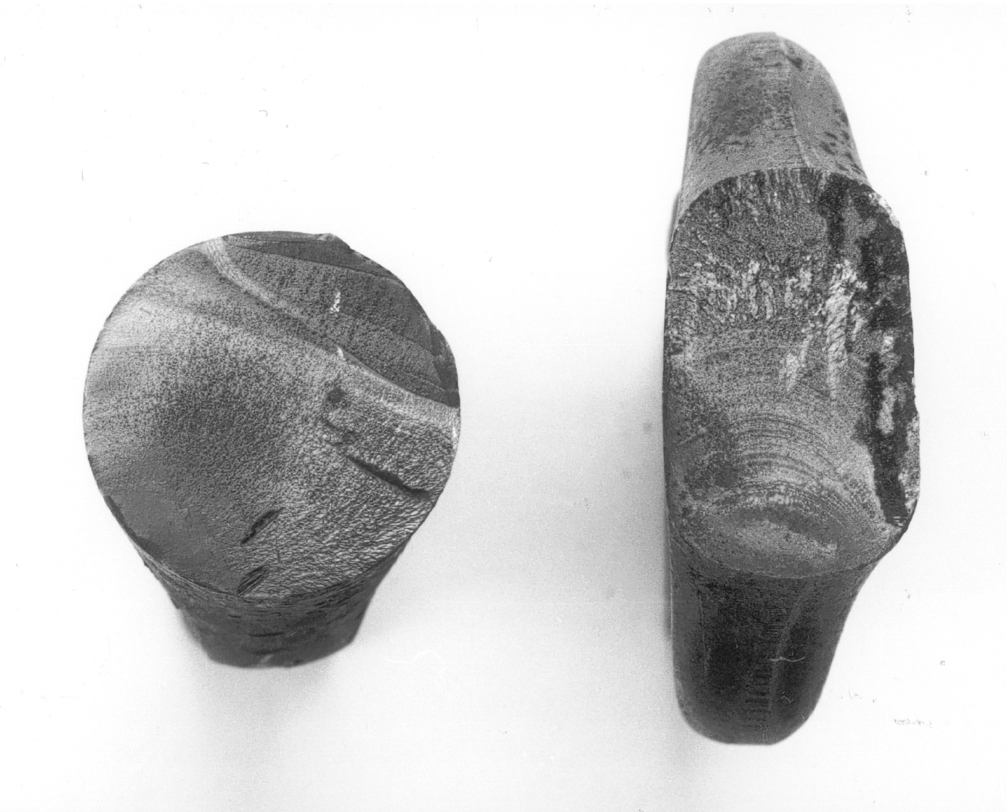
The fatigue crack traverses much more of the cross section in the circular tool than in the rectangular tool. What does this tell you about the maximum stress in the fatigue cycle?
where b and C are constants. Find the number of cycles to failure, Nf, for a component subjected to a stress range of 150 MN m-2.
Answers
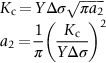
Input Kc = 54, Y = 1.12 and Δσ = 180. This gives a2 = 0.0228 m. Then follow the method of Worked Example 2, integrating from a1 = 0.002 m to a2 = 0.0228 m. This gives 1.15 × 10⁵ cycles.