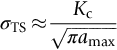
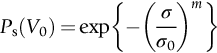
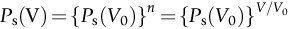
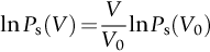
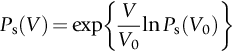
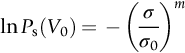
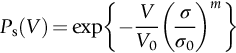
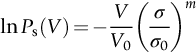
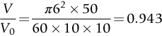
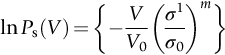
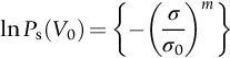
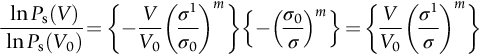
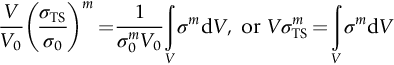
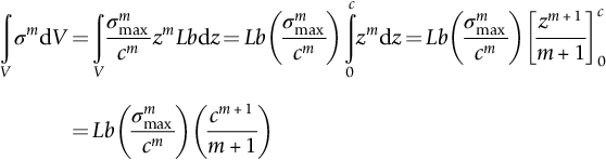
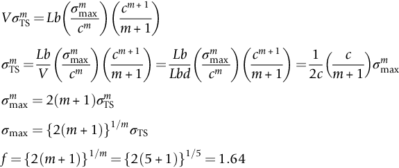
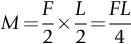
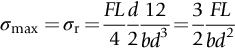
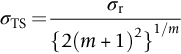
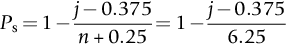
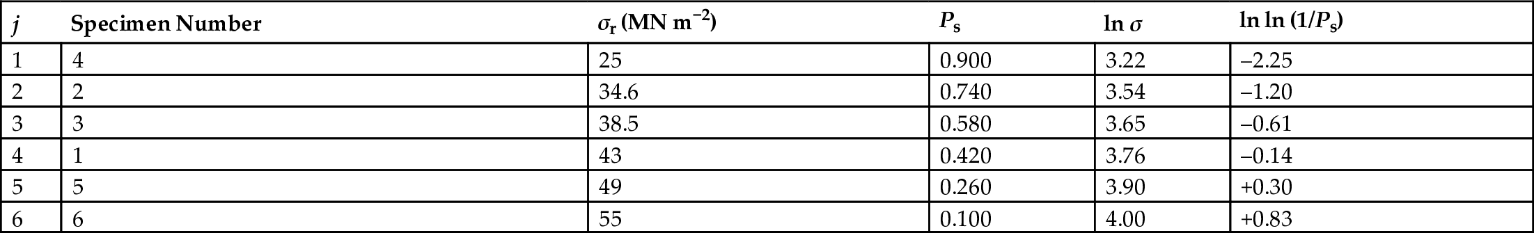
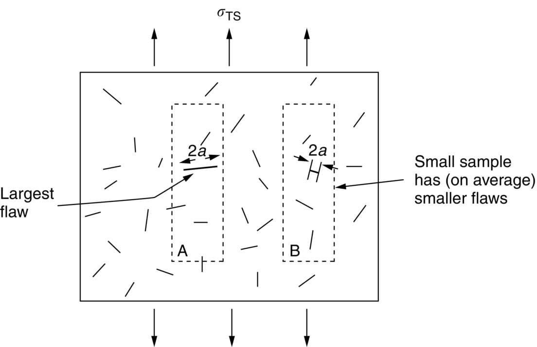
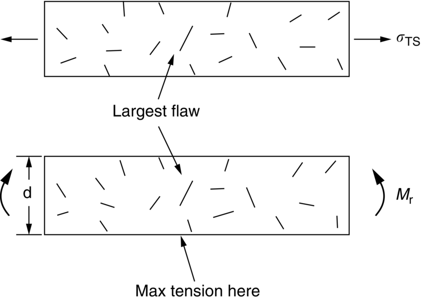
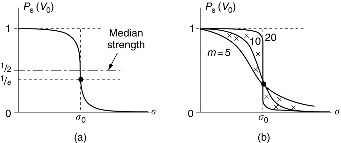
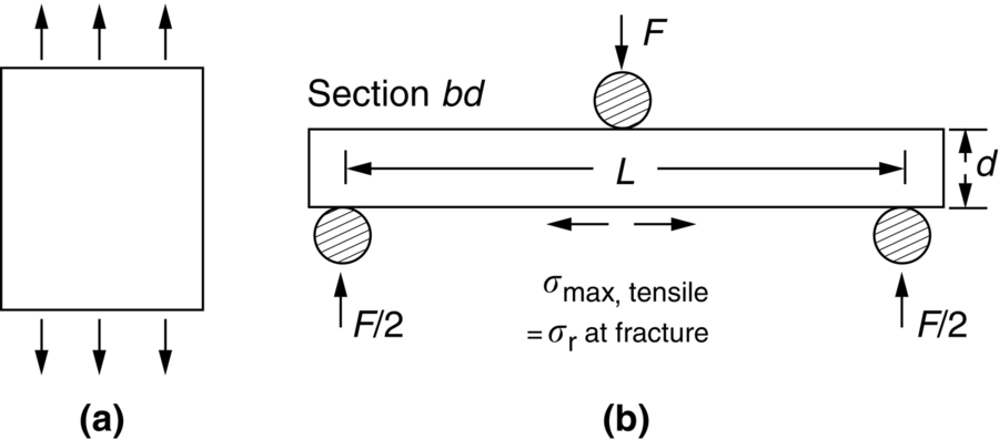
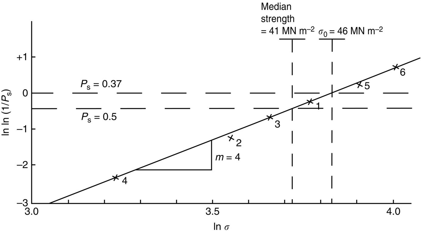
section epub:type=”chapter”> The fracture toughness KC of ceramics and rigid polymers is very low compared to that of metals and composites. Cement and ice have the lowest KC at ≈0.2 MN m −3/2. Even engineering ceramics such as silicon nitride, alumina, and silicon carbide only reach ≈ 4 MNm−3/2. Rigid polymers (thermoplastics below the glass transition temperature or heavily cross-linked thermosets such as epoxy) have Kc ≈0.5–4 MN m−3/2. This low fracture toughness makes ceramics and rigid polymers very vulnerable to the presence of crack-like defects. They are defect-sensitive materials liable to fail by fast fracture from defects well before they can yield. Unfortunately, many manufactured ceramics contain cracks and flaws left by the production process. The defects are worse in cement because of the rather crude nature of the mixing and setting process. Ice usually contains small bubbles of trapped air. Molded polymer components often contain small voids. And all but the hardest brittle materials accumulate additional defects when they are handled or exposed to an abrasive environment. The chapter discusses the probabilistic fracture of brittle materials, the statistics of strength, and the Weibull distribution. The chapter concludes with a discussion of the modulus of rupture. We saw in Chapter 14 that the fracture toughness Kc of ceramics and rigid polymers was very low compared to that of metals and composites. Cement and ice have the lowest Kc at ≈0.2 MN m−3/2. Traditional manufactured ceramics (brick, pottery, china, porcelain) and natural stone or rock are better, at ≈ 0.5–2 MN m−3/2. But even engineering ceramics such as silicon nitride, alumina, and silicon carbide only reach ≈ 4 MN m−3/2. Rigid polymers (thermoplastics below the glass transition temperature, or heavily cross-linked thermosets such as epoxy) have Kc ≈ 0.5–4 MN m−3/2. This low fracture toughness makes ceramics and rigid polymers very vulnerable to the presence of crack-like defects. They are defect-sensitive materials, liable to fail by fast fracture from defects well before they can yield. Unfortunately, many manufactured ceramics contain cracks and flaws left by the production process (e.g., the voids left between the particles from which the ceramic was fabricated). The defects are worse in cement, because of the rather crude nature of the mixing and setting process. Ice usually contains small bubbles of trapped air (and, in the case of sea ice, concentrated brine). Molded polymer components often contain small voids. And all but the hardest brittle materials accumulate additional defects when they are handled or exposed to an abrasive environment. The design strength of a brittle material in tension is therefore determined by its low fracture toughness in combination with the lengths of the crack-like defects it contains. If the longest microcrack in a given sample has length 2amax, then the tensile strength is simply given by from the fast fracture equation. Some engineering ceramics have tensile strengths about half that of steel—around 200 MN m−2. Taking a typical fracture toughness of 2 MN m−3/2, the largest microcrack has a size of 60 μm, which is of the same order as the original particle size. Pottery, brick, and stone generally have tensile strengths that are much lower than this—around 20 MN m−2. This indicates defects of the order of 2 mm for a typical fracture toughness of 1 MN m−3/2. The tensile strength of cement and concrete is even lower—2 MN m−2 in large sections—implying the presence of at least one crack 6 mm or more in length for a fracture toughness of 0.2 MN m−3/2. The chalk with which I write on the board when I lecture is a brittle solid. Some sticks of chalk are weaker than others. On average, I find (to my slight irritation), that about 3 out of 10 sticks break as soon as I start to write with them; the other 7 survive. The failure probability, Pf, for this chalk, loaded in bending under my (standard) writing load, is 3/10, that is, When you write on a board with chalk, you are not unduly inconvenienced if 3 pieces in 10 break while you are using them; but if 1 in 2 broke, you might seek an alternative supplier. So the failure probability, Pf, of 0.3 is acceptable (just barely). If the component were a ceramic cutting tool, a failure probability of 1 in 100 (Pf = 10−2) might be acceptable, because a tool is easily replaced. But if it were the glass container of a cafetiere, the failure of which could cause injury, one might aim for a Pf of 10−4. When using a brittle solid under load, it is not possible to be certain that a component will not fail. But if an acceptable risk (the failure probability) can be assigned to the function filled by the component, then it is possible to design so this acceptable risk is met. This chapter explains why ceramics have this dispersion of strength; and shows how to design components so they have a given probability of survival. The method is an interesting one, with application beyond ceramics to the malfunctioning of any complex system in which the breakdown of one component will cause the entire system to fail. Chalk is a porous ceramic. It has a fracture toughness of 0.9 MN m−3/2 and, being poorly consolidated, is full of cracks and angular holes. The average tensile strength of a piece of chalk is 15 MN m−2, implying an average length for the longest crack of about 1 mm (calculated from Equation (16.1)). But the chalk itself contains a distribution of crack lengths. Two nominally identical pieces of chalk can have tensile strengths that differ greatly—by a factor of 2 or more. This is because one was cut so that, by chance, all the cracks in it are small, whereas the other was cut so that it includes one of the longer flaws of the distribution. Figure 16.1 illustrates this: if the block of chalk is cut into pieces, piece A will be weaker than piece B because it contains a larger flaw. It is inherent in the strength of brittle materials that there will be a statistical variation in strength. There is no single “tensile strength” but there is a certain, definable, probability that a given sample will have a given strength. The distribution of crack lengths has other consequences. A large sample will fail at a lower stress than a small one, on average, because it is more likely that it will contain one of the larger flaws (Figure 16.1). So there is a volume dependence of the strength. For the same reason, a brittle rod is stronger in bending than in simple tension: in tension the entire sample carries the tensile stress, while in bending only a thin layer close to one surface (and thus a relatively smaller volume) carries the peak tensile stress (Figure 16.2). The Swedish engineer, Weibull, invented the following way of handling the statistics of strength. He defined the survival probability Ps(V0) as the fraction of identical samples, each of volume V0, which survive loading to a tensile stress σ. He then proposed that where σ0 and m are constants. This equation is plotted in Figure 16.3(a). When σ = 0 all the samples survive, of course, and Ps(V0) = 1. As σ increases, more and more samples fail, and Ps(V0) decreases. Large stresses cause virtually all the samples to break, so Ps(V0) → 0 and σ → ∞. If we set σ = σ0 in Equation (16.2) we find that Ps(V0) = 1/e (= 0.37). So σ0 is simply the tensile stress that allows 37 % of the samples to survive. The constant m tells us how rapidly the strength falls as we approach σ0 (see Figure 16.3(b)). It is called the Weibull modulus. The lower m, the greater the variability of strength. For ordinary chalk, m is about 5, and the variability is great. Brick, pottery, and cement are like this too. The engineering ceramics (e.g., SiC, Al2O3, and Si3N4) have values of m of about 10; for these, the strength varies much less. Even steel shows some variation in strength, but it is small: it can be described by a Weibull modulus of about 100. Figure 16.3(b) shows that, for m greater than about 20, a material can be treated as having a single, well-defined failure stress. So much for the stress dependence of Ps. But what of its volume dependence? We have already seen that the probability of one sample surviving a stress σ is Ps(V0). The probability that a batch of n such samples all survive the stress is just {Ps(V0)}n. If these n samples were stuck together to give a single sample of volume V = nV0 then its survival probability would still be {Ps(V0)}n. So This is equivalent to or The Weibull distribution (Equation (16.2)) can be rewritten as If we insert this result into equation (16.3) we get or This, then, is our final design equation. It shows how the survival probability depends on both the stress σ and the volume V of the component. In using it, the first step is to fix on an acceptable failure probability, Pf : 0.3 for chalk, 10−2 for the cutting tool, 10−4 for the cafetiere. The survival probability is then given by Ps =1 – Pf. It is useful to remember that, for small Pf, ln Ps = ln (1 – Pf) ≈ – Pf. We can then substitute suitable values of σ0, m, and V/V0 into the equation to calculate the design stress. To test the strength of a ceramic, square section bars measuring 10 by 10 by 60 mm are put into tension along their length. The tensile stress σ that breaks 50% of the bars is 110 MPa. Cylindrical ceramic components 50 mm long with diameter 12 mm are required to take a tensile stress σ1 along their length with a survival probability of 99%. If m = 5, find σ1. This is a simple substitution exercise, writing Equation (16.4) (alternative version) twice, and remembering that when probabilities are given in percentages, they must first be converted to real numbers, in this case 0.5 and 0.99. For the test samples, by definition V = V0, so V/V0 = 1 in Equation (16.4). In the actual component, Using Equation (16.4), we get for the components and for the test samples We then divide the two “ln” terms to give Putting the numbers in, we finally get In this example, the small difference in volume makes essentially no difference to the answer. The reason for the component stress being less than half the test strength is the requirement for the much greater survival probability of 99%.■ Note that Equation (16.4) assumes that the component is subjected to a uniform tensile stress σ. In many applications, σ is not constant, but instead varies with position throughout the component. Then, we rewrite Equation (16.4) as 1. Beams of length L and rectangular cross section b (width) × d (thickness) are subjected to a tensile load along their length. 50% of the beams break when the (uniform) stress in the beam = σTS. 2. Identical beams are then tested in pure bending, as shown in Figure 7.2. 50% of the beams break when the maximum tensile stress in the beam, σmax = f × σTS where f is a dimensionless number. 3. Calculate the value of f if the Weibull modulus m = 5. From Figure 7.2, we can write for the (linear) variation in tensile stress from the neutral axis to the lower surface of the beam. Note that d = 2c. For case (1) Equation (16.4) gives For case (2) Equation (16.5) gives Since Ps(V) = 0.5 for both cases, we can equate the two equations, to give We take a volume element dV, which is a thin strip of material length L, width b, and thickness dz, which lies between the neutral axis and the lower surface of the beam, and is parallel to the neutral axis. dV = Lbdz. Then ■ Note that we only integrate over the lower half of the beam in the bending case—the upper half is in compression, so cracks there should not cause failure. The beam is much stronger in pure bending than in simple tension because in bending, one half of the beam is neglected; the stress in the other half varies linearly from zero to σmax, so the stress exceeds σTS only in a relatively small volume. This type of analysis is not difficult—it’s just tedious, and care needs to be taken to avoid silly slips. There is much canceling through of terms to be done, and if the final equation does not reduce to a fairly elegant dimensionless ratio, then something has probably gone wrong! In Chapter 9 we saw that properties such as the yield and tensile strengths could be measured easily using a long cylindrical specimen loaded in simple tension. But it is difficult to perform tensile tests on brittle materials—the specimens tend to break where they are gripped by the testing machine. This is because the local contact stresses exceed the fracture strength, and premature failure occurs at the grips. It is much easier to measure the force required to break a beam in bending (Figure 16.4). The maximum tensile stress in the surface of the beam when it breaks is called the modulus of rupture, σr. Using the results for the elastic bending of a beam in Chapter 7, we can easily find the modulus of rupture from the load F and the dimensions of the specimen L, b, and d. From Figure 7.2, we can see that the stress at the surface of a beam is given by From Figure 16.4, we can see that at the midspan of the beam (L/2). From Figure 7.4, we can see that the second moment of area for the beam cross section is given by Comparing Figures 7.2 and 16.4 tells us that Combining equations, we get for the modulus of rupture, σr.■ You might think that σr; should be equal to the tensile strength σTS. But it is actually larger than the tensile strength. There are two reasons for this. The first is that half of the beam—the half above the neutral axis—is subjected to compressive stresses. Flaws here will close up, and will be very unlikely to propagate to failure. The second is that the peak tensile stress is located in the lower surface of the beam, vertically below the loading point. Everywhere else, the tensile stress is lower—in many cases much lower. So only a small volume is subjected to high tensile stress. The tensile strength may be found from the modulus of rupture using the following equation: This is derived using Equation (16.5), together with the (known) stress state in the beam. For example, if m = 10, σTS = σr/1.73. If m = 5, σTS = σr/2.35. How do we find σ0, m, and the median strength from test data? The table gives results from a set of six separate bend tests (numbered 1–6). Listed for each specimen is the maximum tensile stress at mid-span when fracture occurred—the modulus of rupture, calculated using Equation 16.6. Note that the initiating flaw was not always located at the position of maximum tensile stress. The table ranks the test results in order of increasing modulus of rupture (j = 1 to 6). Then Ps can be found from the standard statistical result Values for Ps are listed in this table. The trick for analyzing the data is as follows. We start with the basic Weibull equation—Equation (16.2)—for specimens all having the same volume V0. Taking natural logs on each side of Equation (16.2), we get Taking natural logs on each side again gives Note that the last term in this equation is a constant. The preceding table lists values for ln ln (1/Ps) and ln σ, and these are plotted in the following diagram. The slope of the best-fit line is 4 (note that the scales of the vertical and horizontal log axes are not the same!). Therefore, m = 4. We can also easily see that σ0 and the median strength are 46 and 41 MN m−2. This type of graph is called a Weibull plot.
Fracture Probability of Brittle Materials
Publisher Summary
16.1 Introduction
16.2 Statistics of Strength
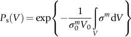
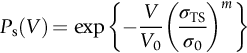
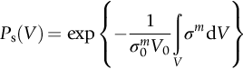
16.3 Weibull Distribution
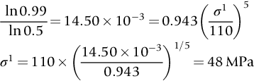
Worked Example 1
Worked Example 2
16.4 Modulus of Rupture
Worked Example 3
Worked Example 4
Examples
 . You may assume that the volume of a cone is given by
  .
.
Explain why there is a dependency on cone angle α, even though the stress variation up the stalactite is independent of α.
Answers