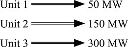
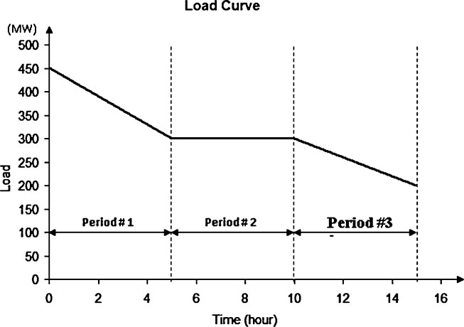
The reliability studies depend on a number of indices. These indices are defined in the previous chapters and in the coming chapters (Kim, 2011; Rusin and Wojaczek, 2015). In the present chapter, a number of indices explained. The present chapter highlight on loss of load probability (LOLP), expected un-served energy (EUE), loss of load hours (LOLH), loss of load events (LOLEV), expected power not supplied (EPNS), loss of energy probability (LOEP), energy index of reliability (EIR), interruption duration index (IDI), expected energy not supplied (EENS), energy curtailed, loss of load expectation (LOLE), derated state, and forced outage rate (FOR). The electric power system is the most likely complex system. The system divided into functional areas. These areas called generation, transmission, and distribution. To assess the system reliability, each part to be analyzed separately for easier evaluation and eventually by combining them together. Throughout the period, the resource adequacy metrics explain the occurrence of the risk, which helps the assessment of the power plant. The aggregation of risk across the year of operation might be more suitable to indicate the period of occurrence for resource adequacy risks within the area of operation (IEEE Standard 493–2007). To show the quality and performance of an electrical system, the index LOLP needed. This index value is affected by load growth, the load duration curve, FOR of the plant, number, and capacity of generating units. This index defined as the probability of system as hourly or daily demand exceeding the available generating capacity within a given period. With a daily peak load curve, the LOLP can be calculated. The LOLP is a projected value of how much time the load on a power system is expected to be greater than the capacity of the available generating resources in the end. Therefore, the LOLP is based on combining the probability of generation capacity states with the daily peak probability. Then, as to assess the number of days during the year in which the generation system may be unable to meet the daily peak (Al-Shaalan, 2012; IEEE Standard 493–2007). There are a number of problems that might arise during the use of LOLP of any power system reliability study. These problems are: a. The LOLP does not provide any indication of the duration of shortages or frequency. b. There are different techniques used to find LOLP. These techniques might obtain a different result for the same system. c. The LOLP does not include additional emergency support that one control area may receive from another, even though any region does not include the additional emergency. d. As a result of a future event not modeled by traditional LOLP calculation, major loss of load incidents usually occur. e. The use of the LOLP index would be sufficient for the same system to investigate different expansion plans and an annual maintenance schedule. This is an argue statement and at the same time, it is correct only in case the duration peak load is static over any number of years of the study. f. In the case that the utilities have different shapes of load curve, it is not useful to compare the reliabilities of utilities. g. In most often the cumulative curve of any daily peak load, the used load model, which is used in the loss of load method, is not recognized in that model. h. In the case of building the generation or signing purchasing power system equipment agreement, the LOLP is not important as an accurate predictor of the resulting incidence of electricity shortage. i. The LOLP indicates the number of days in a year that might be lost. This indicates that the generation system is not able to meet the required load during those days. This term belongs to the expected unserved energy. This index measures the expected amount of energy that failed to supply during the period of observation of the system load cycle due to shortages of basic energy supplies. In another way, it can be defined as a measure of the resource availability to serve the required load continuously at delivery points. It can be defined as the expected energy required that will not serve in a given year. The EUE can provide a measure relative to the size of a given assessment area (Billinton and Allan, 1996; IEEE Standard 493–2007). At the same time, the expected number of hours per year can be known as the LOLH when a system’s hourly demand is exceeding the generating capacity. This index can be calculated from the load duration curve. The hourly LOLE is known as LOLH when considering the latest case. The LOLH has a number of classifications known as annual LOLH, monthly LOLH, and annual EUE, which is known as both actual and at the same time, normalized. In a case that some system load is not served during a period of time annually, this case is called LOLEV (NERC, 2016). The event might be an hour or a number of hours. At the same time, this is defined as the number of events where some system load is not served in through the year. A LOLEV can last for one hour or for several number of hours and can involve the loss of one or several hundred megawatts of load. This is known as the frequency of occurrence index (Billinton and Allan, 1996). The EPNS (Elsaiah et al., 2015) is equivalent to the required curtailment since the problem aims to minimize the total load curtailment (Billinton and Allan, 1996). The EPNS is estimated as where: i is the number of cases; LOL is the loss of load. Loss-of-energy probability is a measure for generation reliability assessment (Gold Book, 2007). As a relationship, the LOEP is the ratio of the expected energy not served (EENS) during a certain long period of observation to the total energy demand during the same period (Billinton and Allan, 1996). Using the load duration curve is helping to calculate the LOEP for installed capacity. Therefore, the LOEP is becoming as where the LOEP is unitless and it is a probability; Ei is the energy and it is not supplied due to a capacity outage (Oi); Pi is the probability of the capacity outage (Oi); E during the period of study, and E is the total energy demand. The EIR (Venkatamuni and Reddy, 2014) is given by: where EENS is the expected energy not supplied (Billinton and Allan, 1996). The IDI (Florencias-Oliveros et al., 2018) and (Indiana Utility Regulatory Commission Report) is defined as the IDI (Billinton and Allan, 1996). At the same time, the customer average interruption duration index (CAIDI). The term EENS (or Not Served) is the energy, which is needed to satisfy the load based on the generating units available. In other words, when the load exceeds the available generation, it is called EENS. This means that the energy is reflecting risk. The suitable unit used for the EENS is MWhr per year (Al-Shaalan, 2012; Billinton and Allan, 1996). Example (6.1): Consider the load duration curve shown below. This curve represents a variation of the load duration curve (Figure 6.1) of a small power network. Three units are running to satisfy the above load curve, where the capacities of the units are: Find the EENS for the three periods shown on the curve. Solution: Period #1: To satisfy the first period presented in the curve, the generating-units (2 and 3) are running. Running the second and the third units with their full capacities will keep the network under risk. For this reason, the three units should be running. Period #2: To be in the safe side, the units 1 and 3 can be run together (50MW, 300 MW) Period #3: Units 1 and 3 can be run together (50 MW, 300 MW) If all units (1, 2, and 3) are off, then the EENS will be the total area under the curve. EENS = 1875 + 1500 + 1250 = 4625 MW.hr Unit # Period # 1 2 3 1 OFF ON ON 2 ON OFF OFF 3 ON ON ON
CHAPTER 6
Generating Systems Reliability Indices
6.1 INTRODUCTION
6.2 PROBABILISTIC INDICES
6.2.1 LOSS OF LOAD PROBABILITY (LOLP)
6.2.2 EXPECTED UN-SERVED ENERGY (EUE) AND LOSS OF LOAD HOURS (LOLH)
6.2.3 LOSS OF LOAD EVENTS (LOLEV)
6.2.4 EXPECTED POWER NOT SUPPLIED (EPNS)
6.2.5 LOSS OF ENERGY PROBABILITY (LOEP)
6.2.6 ENERGY INDEX OF RELIABILITY (EIR)
6.2.7 INTERRUPTION DURATION INDEX (IDI)
6.2.8 EXPECTED ENERGY NOT SUPPLIED (EENS)
6.2.9 ENERGY CURTAILED
Due to a shortage in energy where the reason behind is that the demand for electricity exceeds the available power is known as curtailment. Therefore, the term curtailment is one among many tools to maintain system energy balance. It should be known that there are hierarchies of customers. This type of hierarchy is clear where some might require a partial or total cut back of electricity before others. The industrial sectors (industrial customers) are usually curtailed before reducing the service to the residential customers. When electrical energy service has to be interrupted, it means that energy reserves have dropped or are expected to drop below a certain level (Billinton and Allan, 1996; Denholm and Mai, 2019; IEEE Standard 493–2007; Schermeyer et al., 2018).
Example (6.2):
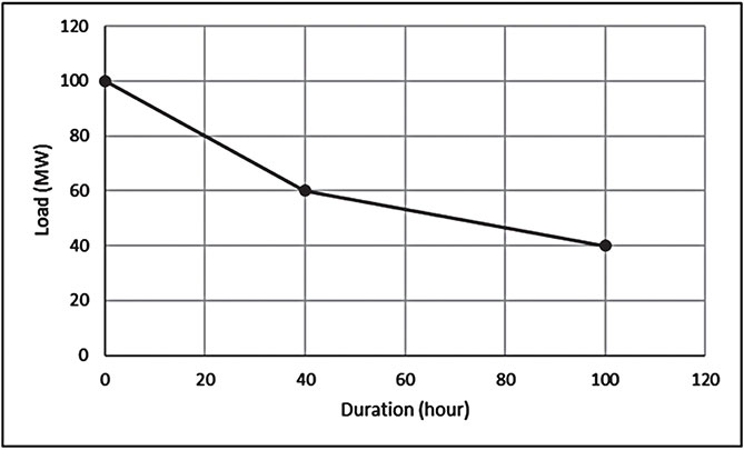
Consider a small electric power system network represented by a load duration curve shown in Figure 6.2. The load curve is represented for a period of 100 hours. The network is running by a generating unit through three-states shown in Table 6.1. Calculate the Energy Curtailed for the considered case. Then, find the generating-unit expected produced energy.
Capacity IN (MW) | Capacity OUT (MW) | Probability |
|---|---|---|
50 | 0 | 0.65 |
30 | 10 | 0.30 |
0 | 25 | 0.05 |
Solution:
First, the total energy under the curve is calculated as:
Therefore, the expected energy produce by the unit-generator is the difference between energy under the curve (EENS0, the generating unit or units is/are OFF) and the summation of the expectation of energy curtailed. This means that the generating-unit expected produced energy is 4150 MWhr.
Capacity IN (MW) | Capacity OUT (MW) | Probability | Energy Curtailed (MWhr) | Expectation of E. C. (MWhr) |
|---|---|---|---|---|
50 | 0 | 0.65 | 6200–(100×50) = 1200 | 0.65×1200 = 780 |
30 | 10 | 0.30 | 6200–(100×30) = 3200 | 0.30×3200 = 960 |
0 | 25 | 0.05 | 6200–(100×0) = 6200 | 0.05×6200 = 310 |
∑ = 2050 MWhr |
Example (6.3):
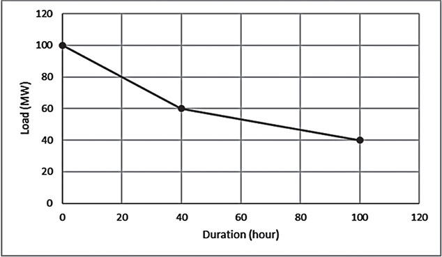
Consider a small electric power system network represented by a load duration curve shown in Figure 6.3. The load curve is represented for a period of 100 hours. The network is running by two-generating units through the three-state model and two-state model as shown in Tables 6.2 and 6.3. Calculate the energy curtailed for the considered case. Then, find the generating-units expected produced energy.
Cap. IN (MW) | Cap. OUT (MW) | Probability |
|---|---|---|
25 | 0 | 0.65 |
15 | 10 | 0.3 |
0 | 25 | 0.05 |
Cap. IN (MW) | Cap. OUT (MW) | Probability |
|---|---|---|
30 | 0 | 0.97 |
0 | 30 | 0.03 |
Solution:
First, the total energy under the curve is calculated as:
The results are shown in Tables 6.4 and 6.5.
Cap. IN (MW) | Cap. OUT (MW) | Prob. | Curtailed Energy | Expectation of E. C. (MWhr) |
|---|---|---|---|---|
25 | 0 | 0.65 | 3700 | 2405 |
15 | 10 | 0.3 | 4700 | 1410 |
0 | 25 | 0.05 | 6200 | 310 |
The total expectation of energy curtailed = 4125 MWhr
Cap. IN (MW) | Cap. OUT (MW) | Prob. | Curtailed Energy (MWhr) | Expectation of E. C. (MWhr) |
|---|---|---|---|---|
30 | 0 | 0.97 | 3200 | 3104 |
0 | 30 | 0.03 | 6200 | 186 |
The total expectation of energy curtailed = 3290 MWhr
Joining both generating-units together:
Cap. IN (MW) | Cap. OUT (MW) | Prob. | Energy Curtailed (MWhr) | Expectation (MWhr) | Connect |
|---|---|---|---|---|---|
55 | 0 | 0.6305 | 700 | 441.35 | 25 + 30 |
45 | 10 | 0.291 | 1700 | 494.7 | 15 + 30 |
30 | 25 | 0.0485 | 3200 | 155.2 | 0 + 30 |
25 | 30 | 0.0195 | 3700 | 72.15 | 25 + 0 |
15 | 40 | 0.009 | 4700 | 42.3 | 15 + 0 |
0 | 55 | 0.0015 | 6200 | 9.3 | 0 + 0 |
Σ 1 | Σ 1215 MWhr |
6.2.10 LOSS OF LOAD EXPECTATION (LOLE)
The term LOLE is one of the reliability indices. During the observation of the power system load cycle, the expected number of hours (HLOLE: Hourly Loss of Load Expectation) or time period are calculated when insufficient generating capacity is available to serve the required load at a time. In another statement, it can be defined as the expected number of days per annual period in which the available generation capacity is insufficient to satisfy and serve the daily maximum load. It can be calculated from the daily peak load or annual peak load. In practical applications, the LOLE expectation index is more often used than the LOLP probability index. The relationship between both the LOLP and the LOLE is formulated as (IEEE Standard 493–2007):
In case the load model is an annual continuous load curve with day maximum load, then the LOLE unit is in days per year and T = 365 days.
In case the load model is an hourly load curve, then the LOLE unit is in hours per year and T = 8760 hours.
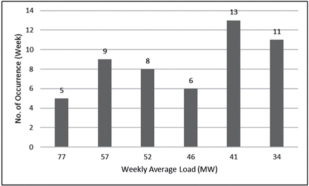
Example (6.4):
A power station is supplying a city in the Kingdom of Bahrain for a year. The weekly average loads have been recorded as such (in MW):
77 | 46 | 41 | 52 |
34 | 41 | 34 | 41 |
41 | 34 | 41 | 57 |
41 | 46 | 57 | 77 |
41 | 52 | 34 | 34 |
57 | 46 | 77 | 41 |
52 | 57 | 41 | 34 |
41 | 41 | 52 | 57 |
34 | 57 | 34 | 52 |
41 | 77 | 34 | 34 |
57 | 52 | 57 | 46 |
77 | 46 | 52 | 34 |
57 | 41 | 52 | 46 |
The power station supplying the city has three generating units, the first unit is working with a capacity of 25MW and 0.02 fail per week. The second unit has a capacity of 25 MW as well, with a failure rate equal to 0.05 f/week. The last unit (number 3) has a repair rate of 0.96 r/week, and its capacity is 50 MW. Calculate the LOLE in percentage.
Solution:
Weekly Average Load (MW) | 77 | 57 | 52 | 46 | 41 | 34 |
No. of Occurrence (week) | 5 | 9 | 8 | 6 | 13 | 11 |
Unit # | Capacity (MW) | Prob. of Success | Prob. of Fail |
|---|---|---|---|
1 | 25 | 0.98 | 0.02 |
2 | 25 | 0.95 | 0.05 |
3 | 50 | 0.96 | 0.04 |
|
|
|
|
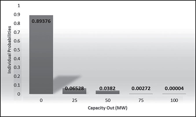
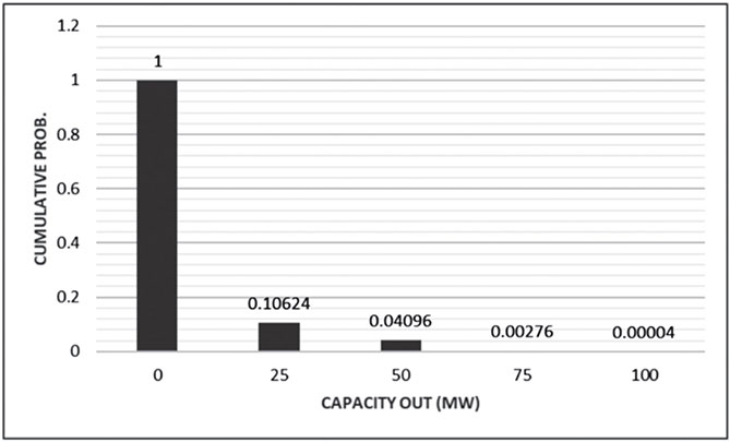
Capacity IN (MW) | Capacity OUT (MW) | Ind. Probability | Cumulative Prob. |
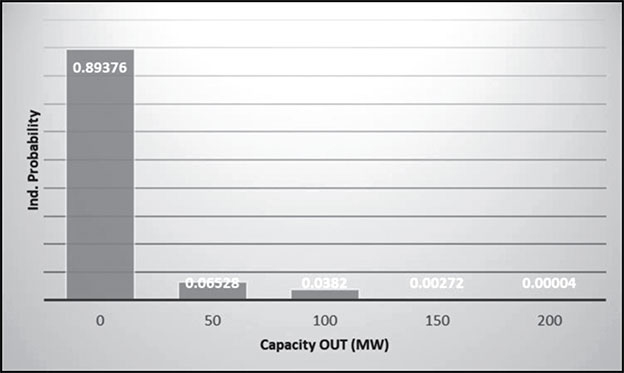
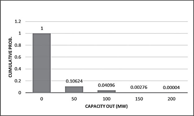
ON-ON-ON 100 | 0 | (0.98)(0.95)(0.96) = 0.89376 | 0.10624 + 0.89376 = 1.00000 |
ON-OFF-ON OFF-ON-ON 75 | 25 | (0.98)(0.05)(0.96)+ (0.02)(0.95)(0.96) = 0.06528 | 0.04096 + 0.06528 = 0.10624 |
OFF-OFF-ON ON-ON-OFF 50 | 50 | (0.02)(0.05)(0.96)+ (0.98) (0.95)(0.04) = 0.0382 | 0.00276 + 0.0382 = 0.04096 |
ON-OFF-OFF OFF-ON-OFF 25 | 75 | (0.98)(0.05)(0.04)+ (0.02) (0.95)(0.04) = 0.00272 | 0.00004 + 0.00272 = 0.00276 |
OFF-OFF-OFF 0 | 100 | (0.02)(0.05)(0.04) = 0.00004 | 0.00004 |
where: the maximum available power is the maximum capacity.
The expected loss of load through the year is approximately equal to 1.3 week. This is equivalent to 9.17 days a year.
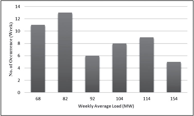
Example (6.5):
A power station is supplying a city in the Kingdom of Bahrain for a year. The weekly average loads have been recorded as such (in MW):
68 | 92 | 82 | 104 |
82 | 114 | 82 | 114 |
92 | 82 | 154 | 68 |
114 | 154 | 114 | 68 |
82 | 114 | 68 | 114 |
82 | 68 | 154 | 104 |
68 | 82 | 114 | 82 |
104 | 82 | 154 | 114 |
114 | 104 | 82 | 92 |
68 | 82 | 104 | 82 |
82 | 68 | 154 | 104 |
92 | 104 | 68 | 92 |
68 | 104 | 92 | 68 |
The power station supplying the city has three generating units, the first unit is working with a capacity of 50MW and 0.02 fail per week. The second unit has a capacity of 50MW as well, with a failure rate equal to 0.05 f/week. The third unit has a repair rate of 0.96 r/week, and its capacity is 100MW. Calculate the LOLE in percentage.
Solution:
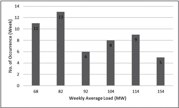
Weekly Average Load (MW) | 68 | 82 | 92 | 104 | 114 | 154 |
No. of Occurrence (week) | 11 | 13 | 6 | 8 | 9 | 5 |
Unit # | Capacity (MW) | Probability of Success | Probability of Fail |
|---|---|---|---|
1 | 50 | 0.98 | 0.02 |
2 | 50 | 0.95 | 0.05 |
3 | 100 | 0.96 | 0.04 |
|
|
|
|
Capacity IN (MW) | Capacity OUT (MW) | Individual Probability | Cumulative Probability |
ON-ON-ON 200 | 0 | (0.98)(0.95)(0.96) = 0.89376 | 0.10624 + 0.89376 = 1.00000 |
ON-OFF-ON OFF-ON-ON 150 | 50 | (0.98)(0.05)(0.96)+ (0.02) (0.95)(0.96) = 0.06528 | 0.04096 + 0.06528 = 0.10624 |
OFF-OFF-ON ON-ON-OFF 100 | 100 | (0.02)(0.05)(0.96)+ (0.98) (0.95)(0.04) = 0.0382 | 0.00276 + 0.0382 = 0.04096 |
ON-OFF-OFF OFF-ON-OFF 50 | 150 | (0.98)(0.05)(0.04)+ (0.02) (0.95)(0.04) = 0.00272 | 0.00004 + 0.00272 = 0.00276 |
OFF-OFF-OFF 0 | 200 | (0.02)(0.05)(0.04) = 0.00004 | 0.00004 |
where: the maximum available power is the maximum capacity.
The expected loss of load through the year is approximately equal to 1.3 week. This is equivalent to 9.17 days a year.
Example (6.6):
Three generators have been running for 52 weeks. These generators are represented by the following data summarized in the following table:
Unit # | Capacity (MW) | Prob. of Success | Prob. of Fail |
|---|---|---|---|
1 | 50 | 0.998 | 0.002 |
2 | 60 | 0.995 | 0.005 |
3 | 100 | 0.992 | 0.008 |
The table below shows the data of the peak loads it occurred and how frequent it is happening:
Weekly Average Load (MW) | 68 | 82 | 92 | 104 | 114 | 154 |
No. of Occurrence (Week) | 11 | 13 | 6 | 8 | 9 | 5 |
Calculate the LOLE in percentage.
Solution:
Capacity IN (MW) | Capacity OUT (MW) | Ind. Probability | Cumulative Prob. |
|---|---|---|---|
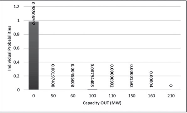
ON-ON-ON 210 | 0 | (0.998)(0.995)(0.992) = 0.98506592 | 1.00000000 |
OFF-ON-ON 160 | 50 | (0.002)(0.995)(0.992) = 0.00197408 | 0.01493408 |
ON-OFF-ON 150 | 60 | (0.998)(0.005)(0.992) = 0.00495008 | 0.01296 |
ON-ON-OFF 110 | 100 | (0.998)(0.995)(0.008) = 0.00794408 | 0.00800992 |
OFF-OFF-ON 100 | 110 | (0.002)(0.005)(0.992) = 0.00000992 | 0.00006584 |
OFF-ON-OFF 60 | 150 | (0.002)(0.995)(0.008) = 0.00001592 | 0.00005592 |
ON-OFF-OFF 50 | 160 | (0.998)(0.005)(0.008) = 0.00004 | 0.00004 |
OFF-OFF-OFF 0 | 210 | (0.002)(0.005)(0.008) = 80 × 10−9 | 80 × 10−9 |
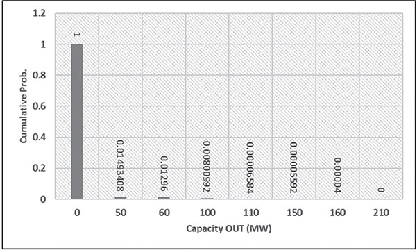
where: the maximum available power is the maximum capacity.
The expected loss of load through the year is approximately equal to 2.77 weeks. This is equivalent to 19.4 days a year.
Example (6.7):
Three generators are running with the following data:
Unit # | Capacity (MW) | λ (f/day) | μ(r/day) |
|---|---|---|---|
1 | 25 | 0.02 | 0.98 |
2 | 25 | 0.03 | 0.97 |
3 | 50 | 0.04 | 0.96 |
The three generators have been running for one year (365 days). The data for a period of one year with a maximum of 100MW are given in the following table:
Daily Peak Load (MW) | 57 | 52 | 46 | 41 | 34 |
No. of Occurrence (days) | 12 | 83 | 107 | 116 | 47 |
Find the LOLE.
Solution:
Unit # | Probability of Success | Probability of Fail |
|---|---|---|
1 | 0.98 | 0.02 |
2 | 0.97 | 0.03 |
3 | 0.96 | 0.04 |
To combine the three units together as one system:
Capacity In (MW) | Capacity Out (MW) | Individual Probability | Cumulative Probability |
|---|---|---|---|
ON ON ON 100 | 0 | (0.98)(0.97)(0.96) = 0.912576 | 0.912576 + 0.087424 = 1.000000 |
ON OFF ON OFF ON ON 75 | 25 | (0.98)(0.03)(0.96)+(0.02)(0.97) (0.96) = 0.046848 | 0.046848 + 0.040576 = 0.087424 |
ON ON OFF OFF OFF ON 50 | 50 | (0.98)(0.97)(0.04)+(0.02)(0.03) (0.96) = 0.038600 | 0.038600 + 0.001976 = 0.040576 |
ON OFF OFF OFF IFF ON 25 | 75 | (0.98)(0.03)(0.04)+(0.02)(0.97)(0.04) = 0.019520 | 0.019520 + 0.000024 = 0.001976 |
OFF OFF OFF 0 | 100 | (0.02)(0.03)(0.04) = 0.000024 | 0.000024 |
where: the maximum available power is the maximum capacity.
Daily Peak Load (MW) | 57 | 52 | 46 | 41 | 34 |
No. of Occurrence (days) | 12 | 83 | 107 | 116 | 47 |
This figure shows that the system might loss power for 4.38824 days in a year. This means that the expected number of hours per year that the system’s electricity production cannot meet its demand.
The loss of load percentage = (4.38824 / 365) × 100 = 1.2327%
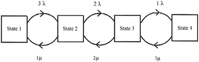
6.2.11 DERATED STATE
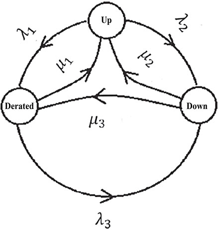
Usually, the term derating is used in the electric power systems and electronic devices. At the same time, the derating as a term used when a component rated less than the maximum capability of it. In the field of electric power systems, the expected excess of available generation capacity over electric power demand is known as the derated capacity margin (Billinton and Allan, 1992; IEEE Standard 493–2007). The de-rated capacity margin statement is used; because uncontinuous plant generation depending on weather conditions, and at the same time, the plants provide uncertain levels of generation capacity. At a case of some generating-units at non-peak demand times are under maintenance, the system could be considered under the derated state. As an example, the three-state model is considered as shown in Figure 6.4. This model has the following states:
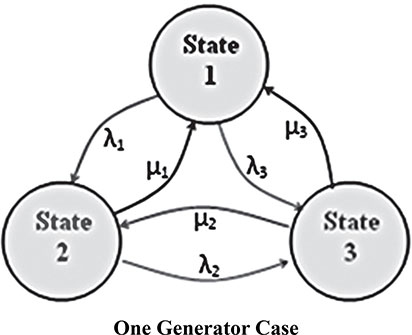
• State (1): it means that the system is operated with full capacity.
• State (2): it means that the system is working with the partial of its capacity (which is defined as a derated-state).
• State (3): it means that the system is in the fail state.
Therefore,
6.2.12 FORCED OUTAGE RATE (FOR)
This index varies between the resource types and areas. The FOR can be also defined in a formula shape as (Billinton and Allan, 1992; IEEE Standard 493–2007):
6.2.13 AVAILABILITY AND UNAVAILABILITY
The availability (Davidov and Pantos, 2019) of the system has a number of formulas:
At the same time, when the system has two-states the availability of the system is given by
In case, the system has three states: up-state, derated-state, and downstate. Therefore,
This means the availability is considered that the system is under operation. The unavailability means that the system is in the fail state.
6.3 GENERATION SYSTEM RELIABILITY EVALUATION (MEASUREMENT)
Any power system is evaluated based on a number of points, these points are summarized as (Akhavein and Porkar, 2017; Al-Shaalan, 2012; Chaiamarit and Nuchprayoon, 2013; Zhong et al., 2017):
a. The unit(s) availability during the operation time.
b. The unit(s) unavailability during the operation time.
c. The system components, which are classified as repairable or non-repairable.
d. The components might be in service or out of service.
e. The state probabilities need to known.
f. The load forecast during the electric network operation.
6.3.1 GENERATION AND LOAD MODELS
The generation model (Ma et al., 2018; Staveley-O’Carroll, 2019) is represented in its simplest form, which is a two-state model. This means that it will pass through the up-state and down-state. This case has been discussed earlier. The load model (Wang et al., 2018; Lv et al., 2018; Zheng et al., 2019) is represented by the load curve.
6.3.2 SYSTEM RISK INDICES
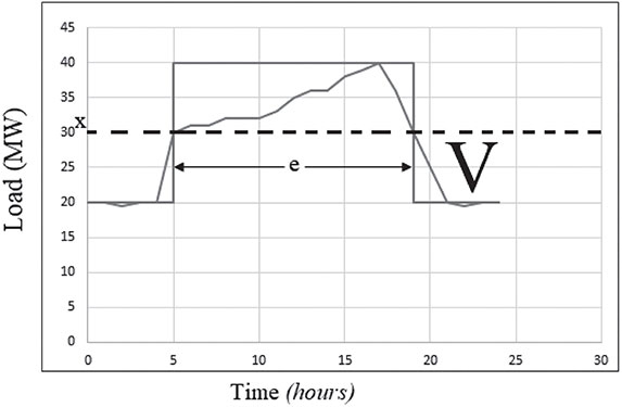
A combination of the generating capacity and the load models will result in the system risk indices. A random sequence of N number of load levels is known as a load cycle for the period (Mosaad et al., 2018; Yu et al., 2018). The N number of load periods must be an integer. As an example, if a daily load model has a peak load level of mean duration e day (e is known as the exposure factor) and a fixed low load of (1 – e) day. The electric load exposure factor is represented in the impact of the risk over the load asset, or percentage of load asset lost. As an example, if the load asset value is reduced two thirds, the load exposure factor value is 0.667. If the asset is completely lost, the exposure factor is unity. Therefore, this case can be represented as a daily load model curve as illustrated in Figure 6.5.
With reference to Figure 6.5, the value of X is proportional inversely to the electric load exposure factor (e). This means that when the value of (X) decreases, (e) increases. The electric load cycle can be presented as shown in Figure 6.6.
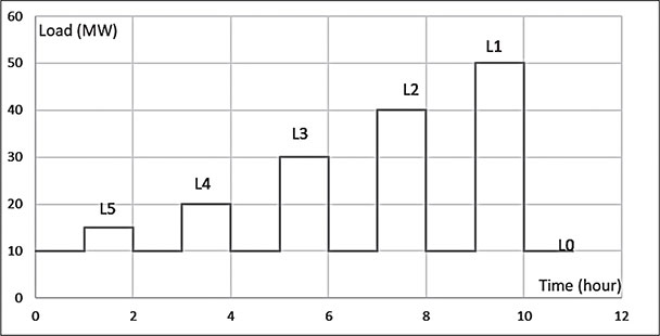
The parameters needed to completely define the load cycle period shown in Figure 6.6 are summarized as shown in Table 6.6.
The combination of discrete levels, the capacity available of the electric system, and discrete levels of electric system demand or electric load form a set capacity margins (mk). It is known that the margin is defined as the difference between the available capacity of the system and the system load. In case that the margin signs is becoming negative. Therefore, it can be concluded that the load is exceeding the available capacity. At this stage, the system might fail. The relationship of such condition can be written in the following form:
and
Item | Parameter(s) |
|---|---|
Number of Load Levels | N |
Peak Electric Loads (MW) | Li, i−1, ………., N such that L1>L2>L3>L4>L5> …….>LN |
Low Electric Load | L0 |
Number of Occurrences of Li | ni, i = 1, ………., N |
Interval Length, hours | |
Mean Duration for the Peak Load | e |
Mean Duration for the Low Load | 1 – e |
Transition Rate to Peak Load (Upward Load) | |
Transition Rate to Peak Load (Downward Load) | |
Transition Rate to Low Load (Upward Load) | |
Transition Rate to Low Load (Downward Load) | |
Frequency of occurrence of Li | |
Frequency of occurrence of L0 | |
Probability of Peak Load | |
Probability of Low Load |
At the same time, departure rates can be written in the following form:
where: λ+m is known as the upward margin rate; λ+C is the upward capacity transition rate; and λ−L is the downward load transition rate.
The probability of the margin state is defined as the product of capacity state and the load state probabilities. It can be written in the following form:
At the same time, a Reserve Margin is the percentage of additional installed capacity through a period that the annual peak demand is recorded. By defining a target generation margin, it is a deterministic criteria used to evaluate system reliability. To calculate the reserve margin, the following equation is used:
As an example (Figure 6.7), consider an electric generation system having 3 × 50MW units, where each unit has a failure rate (λ) of 0.02 f/year and a repair (μ) of 0.48 r/year as shown by the following state-space diagram:
Also, consider for the same system: the variation of a load over a 10 days period (D) scheduled as shown in Table 6.7.
And assume that the exposure factor (e) = 0.5 of a day. Find the capacity margin probability by combining both the generation and load models. The calculations must be on annual basis.
State (i) | Peak Load Level, Li (MW) | No. of Occurrence, ni |
|---|---|---|
1 | 120 | 2 |
2 | 80 | 3 |
3 | 40 | 5 |
In this case, the following solution for the case is followed:
Therefore,
Then, calculating the individual probabilities that the electric power system is passing through using:
The required calculation for the generation model is summarized in Table 6.8, and the load model in Table 6.9.
State | Capacity Out (MW) | Capacity IN (MW) | Individual Probability | Departure Rate | Frequency | |
|---|---|---|---|---|---|---|
λ+n | λ−C | |||||
1 | 0 | 150 | 0.884736 | 0 | 0.06 | 0.053084 |
2 | 50 | 100 | 0.110592 | 0.48 | 0.04 | 0.057507 |
3 | 100 | 50 | 0.004608 | 0.96 | 0.02 | 0.004516 |
4 | 150 | 0 | 0.000064 | 1.44 | 0 | 0.000092 |
State | Peak Load (MW), Li | Number of Occurrence (ni) | Departure Rate | ||
|---|---|---|---|---|---|
λ+L | λ−L | ||||
1 | 120 | 2 | 0.1 | 0 | 2 |
2 | 80 | 3 | 0.15 | 0 | 2 |
3 | 40 | 5 | 0.25 | 0 | 2 |
0 | 0 | λ = 10 | 1 – e = 0.5 | 0 | |
The load model is converted to annual basis. The conversion results are given in Table 6.10.
Probability | |
|---|---|
0.1 | 0.002739 |
0.15 | 0.004109 |
0.25 | 0.006849 |
0.5 | 0.013697 |
Since,
and
At the same time, departure rates written in the following form:
Therefore, the capacity margin and probability calculated as shown in Table 6.11.
Capacity Margin (MW) | Individual Probability |
|---|---|
150 | 0.012118 |
110 | 0.006059 |
100 | 0.001514 |
70 | 0.003635 |
60 | 0.000757 |
50 | 0.000063 |
30 | 0.002423 |
20 | 0.000454 |
10 | 0.000031 |
0 | ≈ 0.0 |
−10 | – |
−20 | 0.000303 |
−30 | 0.000018 |
−40 | – |
Table 6.12 merges the generation and the load shows the results. At the same time, the table shows the construction of margin-availability for the exact margin states. The states illustrated include all combinations of load and capacity.
6.3.3 CAPACITY RESERVE MODEL
In electrical power systems, a balance between supply and demand is expected. For an energy-producer, it refers to the capacity of energy-producer to generate more energy than the system normally requires. This means that a capacity reserve is available. The optimal spinning reserve is considered by the balance between the economy and the reliability of a power system (Li et al., 2019; Xie et al., 2018).
Load | 1 | 2 | 3 | 0 |
|---|---|---|---|---|
Li (MW) | 120 | 80 | 40 | 0 |
Pi | 0.002739 | 0.004109 | 0.006849 | 0.013697 |
λ+L | 0 | 0 | 0 | 2 |
λ −L | 2 | 2 | 2 | 0 |
Generation | ||||
n = 1, C =150 MW | m = 30 | m = 70 | m = 110 | m = 150 |
P1 = 0.884736 | P= 0.002423 | 0.003635 | 0.006059 | 0.012118 |
λ+n = 0 | λ+ = 2 | 2 | 2 | 0 |
λ−n = 0.06 | λ− = 0.06 | 0.06 | 0.06 | 2.06 |
n = 2, C =100 MW | m =−20 | m = 20 | m = 60 | m = 100 |
P2 = 0.116592 | P = 0.000303 | 0.000454 | 0.000757 | 0.001514 |
λ+n = 0.48 | λ+ = 2.48 | 2.48 | 2.48 | 0.48 |
λ−n = 0.04 | λ− = 0.04 | 0.04 | 0.04 | 2.04 |
n = 3, C = 50 MW | m = −70 | m = −30 | m = 10 | m = 50 |
P3 = 0.004608 | P= 0.000012 | 0.000018 | 0.000031 | 0.000063 |
λ+n = 0.96 | λ+ = 2.96 | 2.96 | 2.96 | 0.96 |
λ−n = 0.02 | λ− = 0.02 | 0.02 | 0.02 | 2.02 |
n = 4, C = 0 MW | m = −120 | m = −80 | m = −40 | m = 0 |
P4 = 0.000064 | P = − | – | – | – |
λ+n = 1.44 | λ+ = 3.44 | 3.44 | 3.44 | 1.44 |
λ−n = 0 | λ− = 0 | 0 | 0 | 2 |
6.3.4 EXTENSION TO THE LOSS OF ENERGY CONCEPT
The energy might change from one form to another. Based on that, there will be a loss in that energy. Even though, when it is transformed from one form to another form, there will be some energy loss. This means that when energy is converted to a different form, some of that energy is turned into a highly disordered form of energy. This means that part of that energy will be lost as heat. The main objective of reducing the electricity losses is helping to achieve the goal of universal access to electricity services. Lowering electricity loose-jointed with the greater financial sustainability of utilities. Moreover, lowering the electricity losses is helping to contribute to reduce the air pollution emissions. This means that the electricity losses represent a costly problem in countries and region (Usman et al., 2018).
Two important considerations are known with regard to technical losses. The first technical loss is the availability of power current how it will vary. This means that how much is the current flow through the system. At the same time, the technical losses tend to go up as load increases. The second technical loss is the distance from the source.
6.3.5 PJM METHODS AND MODIFIED PJM
The term PJM is related to Pennsylvania-New Jersey-Maryland Interconnection in the USA (Mid-Atlantic region power pool). The concept remains as a basic method to evaluate unit commitment risk. At the same time, it is used to evaluate the operational reserve requirements. The basic PJM method is followed to evaluate the probability of the committed generation to satisfy of fail to satisfy the expected demand through a period. This means it is used to evaluate the probability to the committed generation. In the end, the method is simplifying the electric power system representation (Billinton and Allan, 1996; Cui et al., 2017; Resource Adequacy Analysis Subcommittee, 2018). The PJM, in its basic form, simplifies the system representation and determines the adequacy of installed capacity requirements using LOLE. In other words, any generating-unit is represented by the two-state model, where the possibility of repair during the lead-time is neglected. It has to take into consideration that the criteria of the PJM are to keep the load in a way that shall not exceed the available capacity. PJM’s capacity market ensures long-term grid reliability. The PJM capacity market is called the Reliability Pricing Model. The PJM is applied as a test system to secure the appropriate amount of power supply resources needed to meet predicted energy demand in the future. In an outage, the probability of finding a two-state model (Figure 6.8) on the outage at a time t:
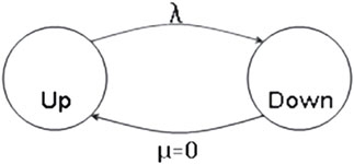
In case, the repair is neglected, the Pdown is becoming:
In cast that λt << 1.
This case is applied for short lead-time to several hours. This is becoming:
This equation representing a generating-unit fails and not replaced by a new unit during the lead-time t. The ORR for each generating-unit is used instead of the FOR.
Example (6.8):
Consider a generating system consists of a number of units; 3 × 20MW, 2 × 30MW, and 3 × 50MW. Assuming that each generating-unit has a failure rate as shown in Table 6.13.
Sub-System | Each Unit (MW) | Number of Unit(s) | Failure Rate (f/year) |
|---|---|---|---|
A | 20 | 2 | 3 |
B | 30 | 3 | 3 |
C | 50 | 2 | 4 |
Calculate the ORR for each case shown in Table 6.13 for lead-times 1, 2, 4 hours.
Solution:
Since the subsystems A and B having the same failure-rate equal 3 f/year, therefore:
This is the ORR for each unit of sub-systems A and B. To calculate the ORR for sub-system C for the same period, which is 1 hour, the ORR becomes:
Following the same procedure to find the ORR for the three sub-systems mentioned earlier. The results are summarized in Table 6.14.
Unit (MW) | Failure Rate (f/year) | ORR (for Lead-Time of Each Sub-System) | ||
|---|---|---|---|---|
1 Hour | 2 Hours | 4 Hours | ||
20 | 3 | 0.000342 | 0.000685 | 0.001370 |
30 | 3 | 0.000342 | 0.000685 | 0.001370 |
50 | 4 | 0.000457 | 0.000913 | 0.001826 |
Example (6.9):
Consider a generating power station consists of a number of units with their failure rates as stated in Table 6.15.
Capacity Unit (MW) | Failure Rate (f/Yr) |
|---|---|
30 | 2 |
20 | 4 |
50 | 4.5 |
40 | 5 |
60 | 5.5 |
55 | 6 |
45 | 6.5 |
35 | 7 |
70 | 8 |
Calculate the ORR for each case shown Table 6.16 for lead-times 1, 2, 3, 4 up to 8 hours. Then, sketch the variation of the ORR and the failure rates.
Solution:
Since,
Therefore, the results are summarized in Table 6.16. The results are represented by the following graph (Figure 6.9).
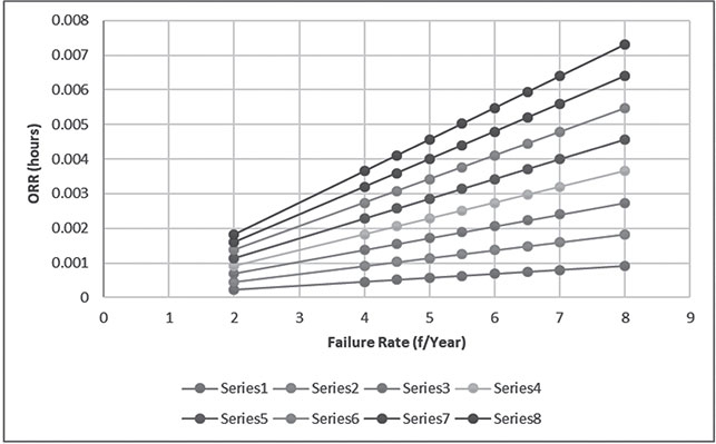
Unit (MW) | Failure Rate (f/Yr) | ORR (hr) | ORR (hrs) | ORR (hrs) | ORR (hrs) | ORR (hrs) | ORR (hrs) | ORR (hrs) | ORR (hrs) |
|---|---|---|---|---|---|---|---|---|---|
1 | 2 | 3 | 4 | 5 | 6 | 7 | 8 | ||
30 | 2 | 0.000228 | 0.000456 | 0.000684 | 0.000913 | 0.001141 | 0.001369 | 0.001598 | 0.001826 |
20 | 4 | 0.000456 | 0.000913 | 0.001369 | 0.001826 | 0.002283 | 0.002739 | 0.003196 | 0.003652 |
50 | 4.5 | 0.000513 | 0.001027 | 0.001541 | 0.002054 | 0.002568 | 0.003082 | 0.003595 | 0.004109 |
40 | 5 | 0.000570 | 0.001141 | 0.001712 | 0.002283 | 0.002853 | 0.003424 | 0.003995 | 0.004566 |
60 | 5.5 | 0.000627 | 0.001255 | 0.001883 | 0.002511 | 0.003139 | 0.003767 | 0.004394 | 0.005022 |
55 | 6 | 0.000684 | 0.001369 | 0.002054 | 0.002739 | 0.003424 | 0.004109 | 0.004794 | 0.005479 |
45 | 6.5 | 0.000742 | 0.001484 | 0.002226 | 0.002968 | 0.003710 | 0.004452 | 0.005194 | 0.005936 |
35 | 7 | 0.000799 | 0.001598 | 0.002397 | 0.003196 | 0.003995 | 0.004794 | 0.005593 | 0.006392 |
70 | 8 | 0.000913 | 0.001826 | 0.002739 | 0.003652 | 0.004566 | 0.005479 | 0.006392 | 0.007305 |
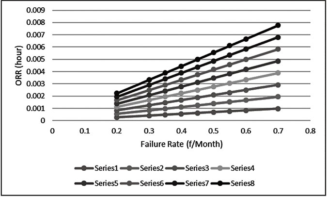
Example (6.10):
Consider a generating power station consists of a number of units with their failure rates as stated in Table 6.17.
Capacity Unit (MW) | Failure Rate (f/Yr) |
|---|---|
30 | 0.2 |
20 | 0.3 |
25 | 0.35 |
40 | 0.4 |
35 | 0.45 |
50 | 0.5 |
55 | 0.55 |
60 | 0.6 |
45 | 0.7 |
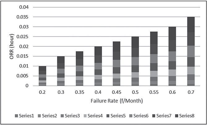
Calculate the ORR for each case shown Table 6.17 for lead-times 1, 2, 3, 4 up to 8 hours. Then, sketch the variation of the ORR and the failure rates. Furthermore, sketch the histogram for the same variables.
Solution:
Since,
Therefore, the results are summarized in Table 6.18, Figure 6.10, and Figure 6.11.
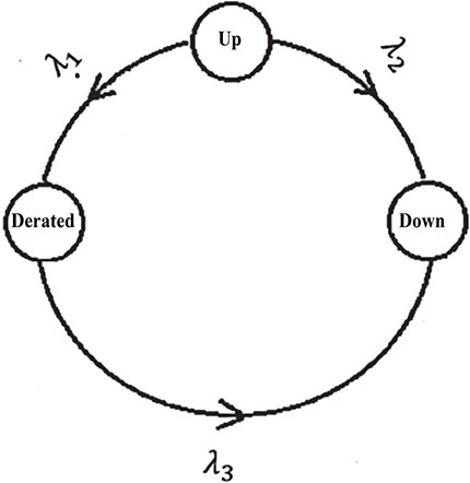
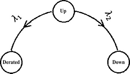
This case of the de-rated state which is called partial output state. This can be illustrated through a system presented as Figure 6.12, where this model can be reduced to Figure 6.13, which shows with a failure rates and no-repair rates. Figure 6.14 represents a model with no transition rates between the de-rated and down states. Figure 6.14 when considered and taking into consideration the assumption that λt << 1, the following probabilities are obtained as:
Failure Rate (f/Month) | ORR (hr) | ORR (hrs) | ORR (hrs) | ORR (hrs) | ORR (hrs) | ORR (hrs) | ORR (hrs) | ORR (hrs) |
|---|---|---|---|---|---|---|---|---|
1 | 2 | 3 | 4 | 5 | 6 | 7 | 8 | |
0.2 | 0.000278 | 0.000556 | 0.000833 | 0.001111 | 0.001389 | 0.001667 | 0.001944 | 0.002222 |
0.3 | 0.000417 | 0.000833 | 0.00125 | 0.001667 | 0.002083 | 0.0025 | 0.002917 | 0.003333 |
0.35 | 0.000486 | 0.000972 | 0.001458 | 0.001944 | 0.002431 | 0.002917 | 0.003403 | 0.003889 |
0.4 | 0.000556 | 0.001111 | 0.001667 | 0.002222 | 0.002778 | 0.003333 | 0.003889 | 0.004444 |
0.45 | 0.000625 | 0.00125 | 0.001875 | 0.0025 | 0.003125 | 0.00375 | 0.004375 | 0.005 |
0.5 | 0.000694 | 0.001389 | 0.002083 | 0.002778 | 0.003472 | 0.004167 | 0.004861 | 0.005556 |
0.55 | 0.000764 | 0.001528 | 0.002292 | 0.003056 | 0.003819 | 0.004583 | 0.005347 | 0.006111 |
0.6 | 0.000833 | 0.001667 | 0.0025 | 0.003333 | 0.004167 | 0.005 | 0.005833 | 0.006667 |
0.7 | 0.000972 | 0.001944 | 0.002917 | 0.003889 | 0.004861 | 0.005833 | 0.006806 | 0.007778 |
The modified PJM means that adding a new component(s) or replacing some by other(s) to satisfy the results or getting better results. The PJM can be extended, because of the assumption that the load can’t be fixed. This means the load from year to year it is expected to increase and vary. Therefore, an estimated technique might be used for future expectations. This expectation needs to make a PJM modification. It is clear, in this case, to extend the system by standby generators or adding for future a new generators to avoid the risk.
6.3.6 RELIABILITY EVALUATION METHODS
To measure the reliability of a model (Gold Book, 2007), the analytical or digital methods are used. There are three methods used to measure the reliability system. These methods are the state space, network reduction, and cut-set methods. The state-space is considered as a general method but becoming cumbersome for large systems. The second method is the network reduction method is applicable for the series and parallel subsystems. The third method (cut-set method) becoming the most popular method. This method used for the transmission and distribution networks (Billinton and Allan, 1996).
6.3.7 DETERMINISTIC METHODS
In an electric power system, spinning reserve requirements can be determined by using deterministic and/or probabilistic methods (Billinton and Allan, 1996).
6.3.8 PLANNING RESERVE MARGIN (PRM)
Planning reserve margin (PRM) used in generation planning (Reimers et al., 2019). The objective of that is to determine an electric utility’s resource. The PRM is used as a figure represents the value of probabilities of electric load occurrence (as an example) in a calculation for system reliability. Furthermore, it is useful in informing resource decisions between reliability indices studies. The peak load is calculated by following several factors. One factor is using the median annual peak load. Another factor is the generation resources, which are subject to forced and planned outages, which might be unavailable during some sometimes through the year when needed. As a third factor, when an interconnection network is available, the utilities hold operating reserves to keep the interconnection network reliable. These factors will keep the network under planning reserves conditions. Therefore, the PRM is well known as the percentage by which the total capacity of system resources exceeds the median peak load. To ensure that the supply of resources to be sufficient to meet load under different system conditions, the surplus capacity is very important.
The capacity reserve margin (CRM) is defined as:
A basic assumption is that enough resources exist to meet the expected load. The PRM is needed for two main reasons; these are the load and resources. The load for a short-term weather-related and Long-term load growth. Regarding the second reason, which is the resources, it depends on three main risks, which are the generation risk, the contract risk, and market risk.
6.3.9 CONTINGENCY RESERVE
The contingency reserve is an appropriation of surplus or retained earnings that may or may not be funded. It indicates a reservation against a specific or general contingency (Motalleb et al., 2016).
6.4 METHOD OF CALCULATION OF INDICES
There are a number of methods to find the indices (Billinton and Allan, 1996). One of which is the Monte Carlo method, which a reliable method and can find the needed indices. At the same time, the method needed in any study is based on the modeling of the different fault clearing technology algorithms considered at the analyses (Honrubia-Escribano et al., 2015).
6.4.1 LOSS OF LOAD PROBABILITY (LOLP, BASIC METHOD)
As explained in section (6.2.1), the LOLP was defined (Boroujeni et al., 2012; Rusin and Wojaczek, 2015; Shirvani et al., 2012). In the present section, it will be illustrated through an example re-calculated referred in reference published by (Boroujeni et al., 2012).
Example (6.11):
Consider a small power plant having two generating-units. Each unit is 100MW with FOR equal to 10%. Find the LOLP for the considered plant that operates to supply 130MW. Then, calculate the number of days of load loss.
Solution:
To find the LOLP, the cumulative probabilities are needed.
No. of Units IN | Capacity IN (MW) | Capacity OUT (MW) | Individual Probability | Cumulative Probability |
|---|---|---|---|---|
2 | 200 | 0 | 0.81 | 1 |
1 | 100 | 100 | 0.18 | 0.19 |
0 | 0 | 200 | 0.01 | 0.01 |
When the power plant is operating at 130MW, it means that the LOLP is the Cumulative Probability of Capacity IN less than the 130MW. This means the LOLP is equal to 0.19 as shown in the above table.
Number of days of load loss, i.e., LOLE = 0.19 × 365 = 69.35 Days/year
Example (6.12):
Consider a power plant having three generators. Each generator is 50MW with FOR equal to 5%. Find the LOLP for the considered plant that operates to supply 120MW. Then, calculate the number of days of load loss.
Solution:
To find the LOLP, the cumulative probabilities are needed.
No. of Units IN | Capacity IN (MW) | Capacity OUT (MW) | Individual Probability | Cumulative Probability |
|---|---|---|---|---|
3 | 150 | 0 | 0.857375 | 1 |
2 | 100 | 50 | 0.135375 | 0.142625 |
1 | 50 | 100 | 0.007125 | 0.00725 |
0 | 0 | 150 | 0.000125 | 0.000125 |
When the power plant is operating at 120MW, it means that the LOLP is the Cumulative Probability of Capacity IN less than the 120MW. This means the LOLP is equal to 0.142625, as shown in the above table.
Number of days of load loss, i.e., LOLE = 0.142625 × 365 = 52.1 days/year
Example (6.13):
In the power system planning (design, operation, and maintenance), reliability is considered as one of the factors that affect. At the same time, athe reliability is divided into adequacy and security. The adequacy relates to the available generation within the system to satisfy the ecustomers demand. Consider the system contains six generating units (Boroujeni et al., 2012) illustrated in Table 6.19. Calculate the probabilities for each company, then merge them to find the probabilities that the system might pass through. How to calculate the LOLP?
Generation Company | Number of Generating-Units | Capacity of Each Generating-Unit (MW) | FOR |
|---|---|---|---|
1 | 2 | 25 | 0.03 |
2 | 2 | 40 | 0.02 |
3 | 1 | 50 | 0.01 |
4 | 1 | 100 | 0.01 |
|
|
|
|
Company (1) | IN (MW) | OUT(MW) | Probability |
2 × 25MW | 50 | 0 | 0.9409 |
25 | 25 | 0.0582 | |
0 | 50 | 0.0009 | |
∑ = 1 | |||
Company (2) | IN (MW) | OUT (MW) | Probability |
2 × 40MW | 80 | 0 | 0.9604 |
40 | 40 | 0.0392 | |
0 | 80 | 0.0004 | |
∑ = 1 | |||
Company (3) | IN (MW) | OUT (MW) | Probability |
1 × 50MW | 50 | 0 | 0.99 |
0 | 50 | 0.01 | |
∑ = 1 | |||
Company (4) | IN (MW) | OUT (MW) | Probability |
1 × 100MW | 100 | 0 | 0.99 |
0 | 100 | 0.01 | |
∑ = 1 | |||
|
|
|
|
Connection(s), IN (MW) | IN (MW) | OUT (MW) | Probability |
50 MW(1) + 80 MW(2) + 50 MW(3) + 100 MW(4) | 280 | 0 | 0.885657917 |
25 MW + 80 MW + 50 MW + 100 MW | 255 | 25 | 0.054782964 |
50 MW + 40 MW + 50 MW + 100 MW | 240 | 40 | 0.036149303 |
(0 MW + 80 MW + 50 MW + 100 MW) & (50 MW + 80 MW + 0 MW + 100 MW) | 230 | 50 | 0.009793199 |
25 MW + 40 MW + 50 MW + 100 MW | 215 | 65 | 0.002236039 |
25 MW + 80 MW + 0 MW + 100 MW | 205 | 75 | 0.000553363 |
50 MW + 0 MW + 50 MW + 100 MW | 200 | 80 | 0.00036887 |
(0 MW + 40 MW + 50 MW + 100 MW) & (50 MW + 40 MW + 0 MW + 100 MW) | 190 | 90 | 0.000399722 |
(0 MW + 80 MW + 0 MW + 100 MW) & (50 MW + 80 MW + 50 MW + 0 MW) | 180 | 100 | 0.008954597 |
25 MW + 0 MW + 50 MW + 100 MW | 175 | 105 | 2.28167E–05 |
25 MW + 40 MW + 0 MW + 100 MW | 165 | 115 | 2.25863E–05 |
25 MW + 80 MW + 50 MW + 0 MW | 155 | 125 | 0.000553363 |
(50 MW + 0 MW + 0 MW + 100 MW) & (0 MW + 0 MW + 50 MW + 100 MW) | 150 | 130 | 4.0788E–06 |
(50 MW + 40 MW + 50 MW + 0 MW) & (0 MW + 40 MW + 0 MW + 100 MW) | 140 | 140 | 0.000365494 |
(0 MW + 80 MW + 50 MW + 0 MW) & (50 MW + 80 MW + 0 MW + 0 MW) | 130 | 150 | 9.89212E–05 |
25 MW + 0 MW + 0 MW + 100 MW | 125 | 155 | 2.30472E–07 |
25 MW + 40 MW + 50 MW + 0 MW | 115 | 165 | 2.25863E–05 |
25 MW + 80 MW + 0 MW + 0 MW | 105 | 175 | 5.58953E–06 |
(50 MW + 0 MW + 50 MW + 0 MW) & (0 MW + 0 MW + 0 MW + 100 MW) | 100 | 180 | 3.72953E–06 |
(50 MW + 40 MW + 0 MW + 0 MW) & (0 MW + 40 MW + 50 MW + 0 MW) | 90 | 190 | 4.0376E–06 |
0 MW + 80 MW + 0 MW + 0 MW | 80 | 200 | 8.6436E–08 |
25 MW + 0 MW + 50 MW + 0 MW | 75 | 205 | 2.30472E–07 |
25 MW + 40 MW + 0 MW + 0 MW | 65 | 215 | 2.28144E–07 |
(50 MW + 0 MW + 0 MW + 0 MW) + (0 MW + 0 MW + 50 MW + 0 MW) | 50 | 230 | 4.12E–08 |
0 MW + 40 MW + 0 MW + 0 MW | 40 | 240 | 3.528E–09 |
25 MW + 0 MW + 0 MW + 0 MW | 25 | 255 | 2.328E–09 |
0 MW + 0 MW + 0 MW + 0 MW | 0 | 280 | 3.6E–11 |
The LOLP is calculated as:
where: Pj is the probability of capacity outage; tj is the percentage of time when the load exceeds Cj; and Cj is the remaining generation capacity.
Appendix (C) illustrates the steps of calculating the LOLP.
6.5 FREQUENCY AND DURATION METHOD
An extension of LOLE is the frequency and duration (F and D) criterion (Billinton and Allan, 1992). The LOLE identifying the expected frequencies of encountering deficiencies and their expected durations. If a fourstate diagram is considered and represented in Figure 6.15, where this diagram is known as a Markov state diagram model.
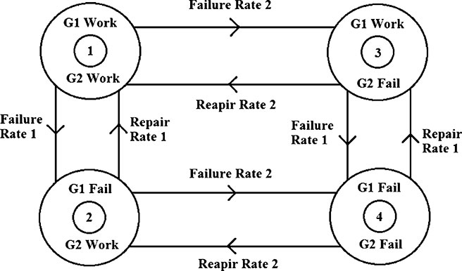
Figure 6.15 represents the four-state model, where the transition rates are defined as:
The steady-state probabilities were calculated in section 5.3.1 for the two-state model. The results of that clear that:
Any Generator in the working-state has a probability equal to:
Therefore, the State-probabilities for the first generator (G1) are:
and the State-probabilities for the first generator (G2) are:
At this stage, the probabilities of the four-state model (Figure 6.15) are calculated as:
The frequency of each state is calculated as follows:
The duration of each state is calculated as follows:
This means the duration in the Up-State becomes:
And the duration in the Down-State is:
6.6 MINIMAL CUT SET METHOD
The cut-set method is applied to a system that has components not connected in a simple form. It means they are not connected in a simple series/parallel form. As an example, the bridge circuit is considered as one form of that type of system. There are two main reasons to use the cut-set technique; these reasons are the simplicity of programming this type of logic network, and the second reason is the cut-set is related directly to the system modes (i.e., failure mode). For this reason, a suitable technique is required for application to solve this type of network. The solution needs to include the conditional probability method, cut, and tie set analysis and logic diagram. The main difference between methods is the logic. The system needs to be reduced to a number of sub-systems following the conditional probability method to reach a suitable solution. Otherwise, failure component(s) might cause a failure of system (Almuhaini and Al-sakkaf, 2017; Billinton and Allan, 1992; Kumar et al., 2017; Rebaiaia and Ait-Kadi, 2013; Zhao et al., 2018).
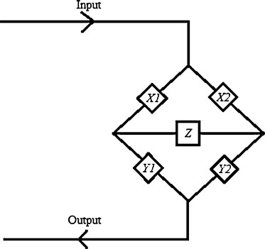
Example (6.14):
Consider a bridge circuit that has five components (X1, X2, Y1, Y2, and Z) connected, as shown in Figure 6.16a. What is the success needs to keep the system in a good condition? And find the overall reliability of the system. Then, assume that the components are identical. Calculate the overall reliability of the system when the reliability of each component is 0.95.
Solution:
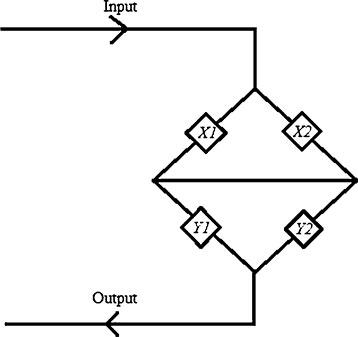
Condition (1): If the component (Z) is good and replaced by a short circuit (allowing the Z to response, i.e., used to give a chance for response passing) as represented by Figure 6.16b. Therefore, the best connections to keep the system under operation are representing the reliability of the system as:
Condition (2): If the component (Z) is bad and replaced by the open circuit (i.e., the component Z does not exist). Therefore, the best connections to keep the system under operation are representing the reliability of the system as:
∴ The overall Reliability of the system (Figure 6.17) is:
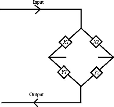
This is the overall system reliability.
When the components are identical, and the reliability of each component is 0.95. Therefore, the overall reliability is:
In case that the reliability of each component is 0.95. Therefore, the overall reliability of the bridge circuit is calculated:
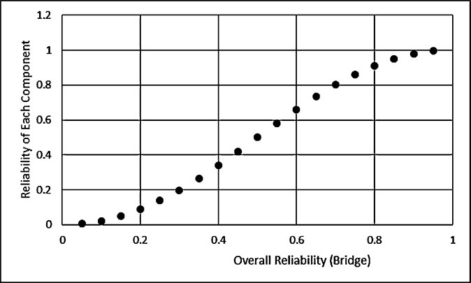
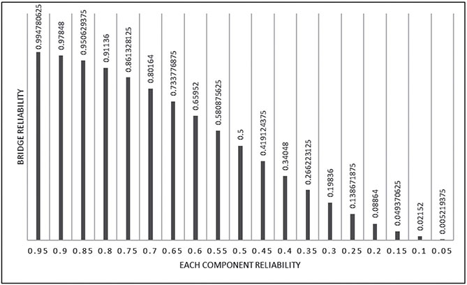
In case that the reliability of each component varies between 0.05 and 0.95 with a step of 0.5. Therefore, the overall reliability becoming as shown in Table 6.20 and drawn as illustrated in both Figures 6.18 and 6.19.
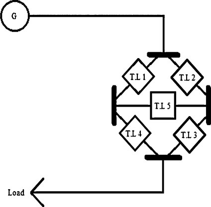
Example (6.15):
Consider a bridge network that has five transmission lines (T.L1, T.L2, T.L3, T.L4, and T.L5). The bridge network fed by a generator connected, as shown in Figure 6.20, and ended by a Load. What is the success needs to keep the system in a good condition? Then, assume that the transmission lines are identical. Calculate the overall reliability of the system when the reliability of each transmission line is 0.95 and the reliability of Generator is 0.91.
Each Component Reliability | Overall System Reliability |
|---|---|
0.95 | 0.994780625 |
0.9 | 0.97848 |
0.85 | 0.950629375 |
0.8 | 0.91136 |
0.75 | 0.861328125 |
0.7 | 0.80164 |
0.65 | 0.733776875 |
0.6 | 0.65952 |
0.55 | 0.580875625 |
0.5 | 0.5 |
0.45 | 0.419124375 |
0.4 | 0.34048 |
0.35 | 0.266223125 |
0.3 | 0.19836 |
0.25 | 0.138671875 |
0.2 | 0.08864 |
0.15 | 0.049370625 |
0.1 | 0.02152 |
0.05 | 0.005219375 |
Solution:
Figure 6.20 is converted to a tie-set diagram as shown in Figure 6.21.
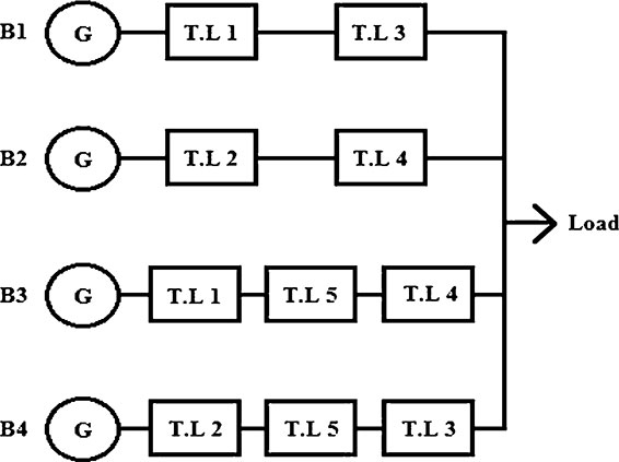
The present example is similar to the previous example (bridge circuit), except that the generator and the load are added to the bridge. Therefore, the bridge network has the overall reliability of the system:
This means that the overall bridge reliability of the bridge is equal to the probabilities of the branches.
Therefore, the overall reliability of the bridge network becoming 0.905250369 and the un-reliability is 0.094749631. The Up-Time of the network is 7929.99323 hours in a year, where the Down-Time of the network is 830.0067698 hours in a year.
In case the network has different values of the generator-reliability and different values of each transmission lines reliability. Therefore, the results are recorded in Table 6.21.
G | TL | Roverall | Qoverall | Up Time (Hour) | Dn Time (Hour) |
|---|---|---|---|---|---|
0.92 | 0.95 | 0.915198175 | 0.084801825 | 8017.136 | 742.864 |
0.95 | 0.99 | 0.949808147 | 0.050191853 | 8320.319 | 439.6806 |
0.94 | 0.98 | 0.939233706 | 0.060766294 | 8227.687 | 532.3127 |
0.93 | 0.97 | 0.928279501 | 0.071720499 | 8131.728 | 628.2716 |
0.92 | 0.96 | 0.916949828 | 0.083050172 | 8032.48 | 727.5195 |
0.91 | 0.95 | 0.905250369 | 0.094749631 | 7929.993 | 830.0068 |
0.9 | 0.94 | 0.89318812 | 0.10681188 | 7824.328 | 935.6721 |
0.89 | 0.93 | 0.880771313 | 0.119228687 | 7715.557 | 1044.443 |
0.88 | 0.92 | 0.868009337 | 0.131990663 | 7603.762 | 1156.238 |
0.87 | 0.91 | 0.854912669 | 0.145087331 | 7489.035 | 1270.965 |
0.86 | 0.9 | 0.8414928 | 0.1585072 | 7371.477 | 1388.523 |
0.85 | 0.89 | 0.827762164 | 0.172237836 | 7251.197 | 1508.803 |
0.84 | 0.88 | 0.813734068 | 0.186265932 | 7128.31 | 1631.69 |
0.83 | 0.87 | 0.799422627 | 0.200577373 | 7002.942 | 1757.058 |
0.82 | 0.86 | 0.784842693 | 0.215157307 | 6875.222 | 1884.778 |
0.81 | 0.85 | 0.770009794 | 0.229990206 | 6745.286 | 2014.714 |
0.8 | 0.84 | 0.754940068 | 0.245059932 | 6613.275 | 2146.725 |
0.79 | 0.83 | 0.739650202 | 0.260349798 | 6479.336 | 2280.664 |
0.78 | 0.82 | 0.724157371 | 0.275842629 | 6343.619 | 2416.381 |
0.77 | 0.81 | 0.708479179 | 0.291520821 | 6206.278 | 2553.722 |
0.76 | 0.8 | 0.6926336 | 0.3073664 | 6067.47 | 2692.53 |
0.75 | 0.79 | 0.676638922 | 0.323361078 | 5927.357 | 2832.643 |
0.74 | 0.78 | 0.660513694 | 0.339486306 | 5786.1 | 2973.9 |
0.73 | 0.77 | 0.64427667 | 0.35572333 | 5643.864 | 3116.136 |
0.72 | 0.76 | 0.627946758 | 0.372053242 | 5500.814 | 3259.186 |
0.71 | 0.75 | 0.611542969 | 0.388457031 | 5357.116 | 3402.884 |
0.7 | 0.74 | 0.595084367 | 0.404915633 | 5212.939 | 3547.061 |
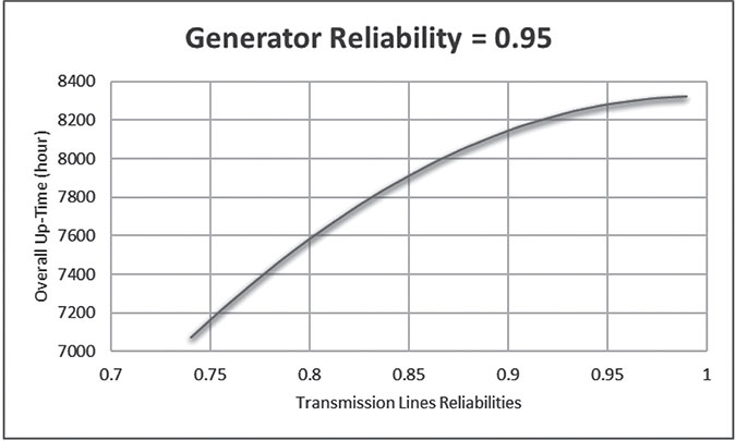
In case that the reliability of the generator is fixed, where the reliability of the identical transmission lines vary as shown in Table 6.22.
G | TL | Roverall | Qoverall | Up Time (Hour) | Dn Time (Hour) |
|---|---|---|---|---|---|
0.95 | 0.95 | 0.945041594 | 0.054958406 | 8278.564 | 481.4356 |
0.95 | 0.99 | 0.949808147 | 0.050191853 | 8320.319 | 439.6806 |
0.95 | 0.98 | 0.949225554 | 0.050774446 | 8315.216 | 444.7841 |
0.95 | 0.97 | 0.948242501 | 0.051757499 | 8306.604 | 453.3957 |
0.95 | 0.96 | 0.946850365 | 0.053149635 | 8294.409 | 465.5908 |
0.95 | 0.95 | 0.945041594 | 0.054958406 | 8278.564 | 481.4356 |
0.95 | 0.94 | 0.942809683 | 0.057190317 | 8259.013 | 500.9872 |
0.95 | 0.93 | 0.940149154 | 0.059850846 | 8235.707 | 524.2934 |
0.95 | 0.92 | 0.937055534 | 0.062944466 | 8208.606 | 551.3935 |
0.95 | 0.91 | 0.933525328 | 0.066474672 | 8177.682 | 582.3181 |
0.95 | 0.9 | 0.929556 | 0.070444 | 8142.911 | 617.0894 |
0.95 | 0.89 | 0.925145948 | 0.074854052 | 8104.279 | 655.7215 |
0.95 | 0.88 | 0.920294482 | 0.079705518 | 8061.78 | 698.2203 |
0.95 | 0.87 | 0.915001802 | 0.084998198 | 8015.416 | 744.5842 |
0.95 | 0.86 | 0.909268973 | 0.090731027 | 7965.196 | 794.8038 |
0.95 | 0.85 | 0.903097906 | 0.096902094 | 7911.138 | 848.8623 |
0.95 | 0.84 | 0.896491331 | 0.103508669 | 7853.264 | 906.7359 |
0.95 | 0.83 | 0.889452775 | 0.110547225 | 7791.606 | 968.3937 |
0.95 | 0.82 | 0.881986542 | 0.118013458 | 7726.202 | 1033.798 |
0.95 | 0.81 | 0.874097689 | 0.125902311 | 7657.096 | 1102.904 |
0.95 | 0.8 | 0.865792 | 0.134208 | 7584.338 | 1175.662 |
0.95 | 0.79 | 0.857075968 | 0.142924032 | 7507.985 | 1252.015 |
0.95 | 0.78 | 0.84795677 | 0.15204323 | 7428.101 | 1331.899 |
0.95 | 0.77 | 0.838442242 | 0.161557758 | 7344.754 | 1415.246 |
0.95 | 0.76 | 0.828540861 | 0.171459139 | 7258.018 | 1501.982 |
0.95 | 0.75 | 0.818261719 | 0.181738281 | 7167.973 | 1592.027 |
0.95 | 0.74 | 0.807614499 | 0.192385501 | 7074.703 | 1685.297 |
Both curves (Figures 6.22 and 6.23) having the same shape, but with a different purpose.
Applying the curve-fitting for the four cases, with a fixed value of the generator-reliability equal to 0.95, the curves are obtained with their formulas:
a. Overall-reliability versus transmission lines reliabilities, represented by Figure 6.24 with the formula:
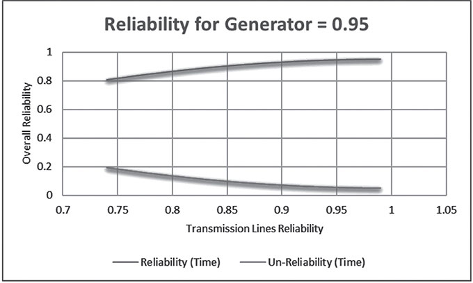
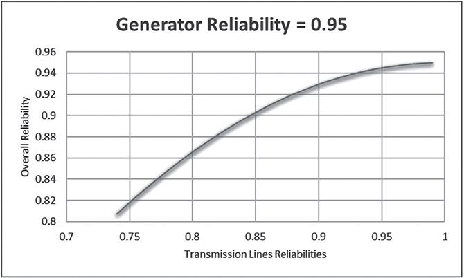
The formula obtained by the curve-fitting and represented as a fourth order polynomial as:
a. = 0.8966963 ± 0.01654
b. = −5,236757 ± 0.07718
c. = 14.10175 ± 0.01346
d. = −12.27874 ± 0.104
e. = 3.467044 ± 0.03006
b. Overall un-reliability versus transmission lines reliabilities, represented by Figure 6.25 with the formula:
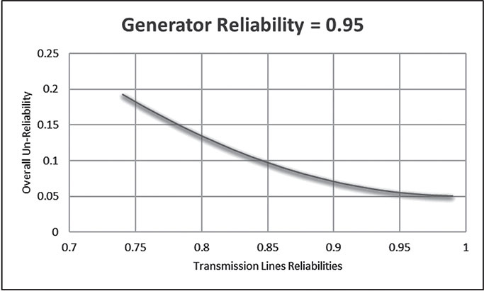
The formula obtained by the curve-fitting and represented as a fourth order polynomial as:
a. = 0.1033037 ± 0.01654
b. = 5.236757 ± 0.07718
c. = −14,101175 ± 0.01346
d. = 12.27874 ± 0.104
e. = −3.467044 ± 0.03006
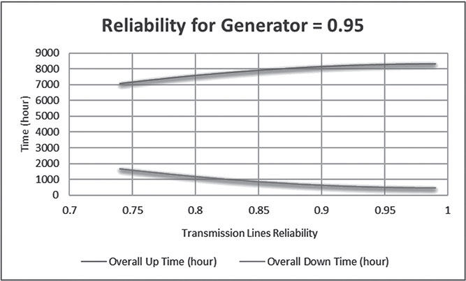
c. Overall up-time versus transmission lines reliabilities, represented by Figure 6.26 with the formula:
The formula obtained by the curve-fitting and represented as a fourth order polynomial as:
a = 7855.051 ± 144.9
b = −45873.95 ± 676.1
c = 123531.2 ± 1179
d = −107561.8 ± 911.3
e = 30371.29 ± 263.3
d. Overall Down-Time versus Transmission Lines Reliabilities, represented by Figure 6.27 with the formula:
The formula obtained by the Curve-Fitting and represented as a Fourth Order Polynomial as:
a. = 904.9481 ± 144.9
b. = 45873.95 ± 676.1
c. = −123531.2 ± 1179
d. = 107561.8 ± 911.3
e. = −30371.29 ± 263.3
These four cases are helping the researcher for more study of such a case of bridge-networks or any type of networks that might need further study.

KEYWORDS
• expected power not supplied
• expected un-served energy
• loss of energy probability
• loss of load events
• loss of load hours
• loss of load probability
REFERENCES
Akhavein, A., & Porkar, B. A composite generation and transmission reliability test system for research purposes. Renewable and Sustainable Energy Reviews, 2017, 75, 331–337.
Almuhaini, M., & Al-Sakkaf, A. Markovian model for reliability assessment of microgrids considering load transfer. Turkish Journal of Electrical Engineering and Computer Sciences, 2017, 25, 4657–4672.
Al-Shaalan, A. M. Reliability evaluation in generation expansion planning based on the expected energy not served. Journal of King Saud University – Engineering Sciences, 2012, 24, 11–18.
Azizah, I. D., Abdullah, A. G., Purnama, W., Nandiyanto, A., & Shafii, M. A. Loss of load probability calculation for west java power system with nuclear power plant scenario. 1st Annual Applied Science and Engineering Conference, IOP Conf. Series: Materials Science and Engineering 180. 2017, 012079. doi: 10.1088/1757–899X/180/1/012079.
Beigvand, S. D., Abdi, H., & Scala, M. L. A general model for energy hub economic dispatch. Applied Energy, 2017, 190, 1090–1111.
Billinton, R., & Allan, R. N. Reliability Evaluation of Engineering Systems: Concepts and Techniques (2nd edn.). Pitman: New York, 1992.
Billinton, R., & Allan, R. N. Reliability Evaluation of Power Systems (2nd edn.). Plenum Press: New York, 1996.
Boroujeni, H. F., Eghtedari, M., Abdollahi, M., & Behzadipour, E. Calculation of generation system reliability index: Loss of load probability. Life Science Journal, 2012, 9(4), 4903–4908.
Chaiamarit, K., & Nuchprayoon, S. Modeling of renewable energy resources for generation reliability evaluation. Renewable and Sustainable Energy Reviews, 2013, 26, 34–41.
Cui, H., Li, F., Fang, X., Chen, H., & Wang, H. Bilevel arbitrage potential evaluation for grid-scale energy storage considering wind power and LMP smoothing effect. IEEE Transactions on Sustainable Energy, 2017.
Davidov, S., & Pantos, M. Optimization model for charging infrastructure planning with electric power system reliability check. Energy, 2019, 166, 886–894.
Denholm, P., & Mai, T. Timescales of energy storage needed for reducing renewable energy curtailment. Renewable Energy, 2019, 130, 388–399.
Elsaiah, S., Benidris, M., & Mitra, J. Reliability-constrained optimal distribution system reconfiguration. Chaos Modeling and Control Systems Design, Studies in Computational Intelligence, 581, Springer International Publishing, Switzerland, 2015. doi: 10.1007/978–3–319–13132–0_11.
Florencias-Oliveros, O., González-De-La-Rosa, J., Agüera-Pérez, A., & Palomares-Salas, J. Discussion on reliability and power quality in the smart grid: A prosumer approach of a time scalable index. International Conference on Renewable Energies and Power Quality (ICREPQ’18), Salamanca (Spain), 2018.
Honrubia-Escribano, A., Giménez, D. U. L., Borroy, V. S., Martín, A. S., & García-Gracia, M. Novel power system reliability indices calculation method. 23rd International Conference on Electricity Distribution, Lyon, Paper 1012, 2015.
IEEE Standard 493–2007. IEEE Recommended Practice for the Design of Reliable Industrial and Commercial Power Systems: Gold Book, 2007.
Indiana Utility Regulatory Commission, Reliability Report Data 2002–2009, Investor-Owned Utilities. Retrieve: www.in.gov/iurc/files/Reliability_Report_Data_2002–2009.pdf (Accessed on 12 October 2019).
Kim, M. C. Reliability block diagram with general gates and its application to system reliability analysis. Annals of Nuclear Energy, 2011, 38, 2456–2461.
Kumar, T. B., Sekhar, O. C., & Ramamoorthy, M. Composite power system reliability evaluation using modified minimal cut set approach. Alexandria Engineering Journal, 2017, Online.
Li, Y., Miao, S., Zhang, S., Yin, B., Luo, X., Dooner, M., & Wang, J. A reserve capacity model of AA-CAES for power system optimal joint energy and reserve scheduling. International Journal of Electrical Power and Energy Systems, 2019, 104, 279–290.
Lv, J., Pawlak, M., Annakkage, U. D., & Bagen, B. Statistical testing for load models using measured data. Electric Power Systems Research, 2018, 163(A), 66–72.
Ma, J., Fouladirad, M., & Grall, A. Flexible wind speed generation model: Markov chain with an embedded diffusion process. Energy, 2018, 164, 316–328.
Mosaad, S. A. A., Issa, U. H., & Hassan, M. S. Risks affecting the delivery of HVAC systems: Identifying and analysis. Journal of Building Engineering, 2018, 16, 20–30.
Motalleb, M., Thornton, M., Reihani, E., & Ghorbani, R. A nascent market for contingency reserve services using demand response. Applied Energy, 2016, 179, 985–995.
Nemes, C. F., & Munteanu, F. A. Probabilistic model for power generation adequacy evaluation. Revue Roumaine des Sciences Techniques-Serie Électrotechnique et Énergétique, 2011, 56(1), 36–46.
North American Electric Reliability Corporation (NERC). Probabilistic Assessment: Technical Guideline Document, 2016.
Rebaiaia, K. L., & Ait-Kadi, D. A New technique for generating minimal cut sets in nontrivial network. AASRI Procedia, 2013, 5, 67–76.
Reimers, A., Cole, W., & Frew, B. The impact of planning reserve margins in long-term planning models of the electricity sector. Energy Policy, 2019, 125, 1–8.
Resource Adequacy Analysis Subcommittee. 11-year planning horizon: June 1st 2018–May 31st 2029 analysis performed by PJM staff, 2018. https://www.pjm.com/-/media/committees-groups/subcommittees/raas/20181004/20181004-pjm-reserve-requirement-study-draft-2018.ashx.
Rusin, A., & Wojaczek, A. Trends of changes in the power generation system structure and their impact on the system reliability. Energy, 2015, 92, 128–134.
Schermeyer, H., Vergara, C., & Fichtner, W. Renewable energy curtailment: A case study on today’s and tomorrow’s congestion management. Energy Policy, 2018, 112, 427–436.
Shirvani, M., Memaripour, A., Abdollahi, M., & Salimi, A. Calculation of generation system reliability index: Expected energy not served. Life Science Journal, 2012, 9(4), 3443–3448.
Staveley-O’Carroll, J. S., & Staveley, O. O. M. International risk sharing in overlapping generations models. Economics Letters, 2019, 174, 157–160.
Systems Operation Division. PJM Manual 40: Training and Certification Requirements, Revision 19, 2018.
Transmission and Distribution System: Electrical Reliability Annual Report, 2015. http://www.keysenergy.com/docs/2018-reliability-report.pdf.
Usman, M., Coppo, M., Bignucolo, F., & Turri, R. Losses management strategies in active distribution networks: A review. Electric Power Systems Research, 2018, 163, 116–132.
Venkatamuni, N. B., & Reddy, B. G. Reliability indices assessment of a small autonomous hybrid power system using aggregate Markov model. Advanced Research in Electrical and Electronic Engineering, 2014, 1(5), 42–47.
Vivek, V., & Prakash, C. Reliability analysis using renewable energy sources. International Journal of Mechanical and Industrial Engineering, 2011, 1(1), 47–50.
Wang, Z., Ji, N., Ma, Y., Liu, Z., & Wang, Y. Model selection mechanism of interactive multiple load modeling. Electrical Power and Energy Systems, 2018, 103, 58–66.
Xie, D., Hui, H., Ding, Y., Lin, Z. Operating reserve capacity evaluation of aggregated heterogeneous TCLs with price signals, Applied Energy, Elsevier, 2018, 216(C), 338–347.
Yu, J., Guo, L., Ma, M., Kamel, S., Li, W., & Song, X. Risk assessment of integrated electrical, natural gas and district heating systems considering solar thermal CHP plants and electric boilers. Electrical Power and Energy Systems, 2018, 103, 277–287.
Zhao, Y., Che, Y., Lin, T., Wang, C., Liu, J., Xu, J., & Zhou, J. Minimal cut sets-based reliability evaluation of the more electric aircraft power system. Hindawi, Mathematical Problems in Engineering, 2018, Article ID 9461823, p. 11. https://doi.org/10.1155/2018/9461823.