6 Geophysical Parameters Estimation
6.1 BAYESIAN ESTIMATION
Parameter estimation has a long history of research and is an ultimate goal in the remote sensing of the Earth’s surface. Multiple parameter estimations from radar measurements becomes a difficult task [1,2]. Several reasons make this so. Because radar echoes are corrupted by noise, this will profoundly, among other factors, affect the accuracy of any parameter estimation. Models that accurately describe the characteristics of radar–surface interactions are usually nonexistent. Well-calibrated in situ measurements, on the other hand, are too small in number to be reliably used. Parameter retrieval from radar returns which are embedded in a noise background are probabilistic in nature. Conventionally, inversion methods, such as those discussed earlier, have been developed to extract a single parameter at a time. However, radar return signals from a natural soil surface are simultaneously affected by surface characteristics such as soil roughness, correlation length, or dielectric constant. It is generally difficult to take hold of the dependence of the measured scattered signal on these parameters within a system limitation. Data enhancement may help to decouple one parameter from another to certain degrees. As a coherent system, radar measurement is always subject to both multiplicative noise and additive noise. We discuss the additive noise first. For radar measurements (observations) that is noisy and may be expressed as
where is “truth” value to be estimated and is noisy and random component.
From the radar equation for a distributed target, Equation 3.38, we see that the received power is the sum of expected signal power and unwanted component, the noise power from system noise: . A good measure to evaluate the impact of noise power on the estimated signal power is the measurement precision [3]:
where are, respectively, the independent samples of the averaged received power and the noise power, and the signal-to-noise ratio, . For most of the system operation, it is set to . The independent samples can be obtained by either spatial sampling or frequency sampling, or both such that , where is the number of spatial samples and is the number of frequency samples. To warrant the spatial samples independence, it is required that , where is the spacing between two measurements corresponding to two different spots within the same distributed targets, and is horizontal correlation length of the surface or volume. The number of frequency-independent samples indeed is the ratio of total system modulation bandwidth to the decorrelation bandwidth. To avoid confusion, in what follows, we shall call N as look number L, though for non-imaging radar measurements such as from scatterometer and altimeter, look number is not as commonly used as in imaging radar.
At this point, it is worth mentioning that estimating from via , (see Equation 3.38), involves several processes, each process, to a different extent, introduces error. For example, solving the integral Equation 3.38 induces error which may be affected by the antenna pattern, the illumination area size, etc. In short, it is affected by the radiometric and geometric properties of the system and of the scene being observed. Note that the integration over an illuminated area overlapping by transmitting and receiving antenna patterns also contributes estimation error. For backscattering and a narrow-beam system, error can be smaller and sometimes ignorable as in many practical applications. Care must be exercised, however, for bistatic measurements at which time-phase-beam synchronizations are critical.
In addition to the additive noise, the inherent multiplicative noise is embedded in the scattering coefficient. For a spatially homogeneous scene with reflectivity variance of within a resolution cell or pixel, the returned radar amplitude follows the Rayleigh distribution, while the returned power follows exponential distribution [1]. The stronger the speckle noise , the wider the distribution, making the estimation of returned power or amplitude more difficult and less accurate. To reduce the speckle strength, more independent samples (look number) of measurement can be made to average down the variance, called multi-looking process, in particular in radar imagery data. If L looks are independent and have equal power, then the distribution of power (intensity) square-law detector is [1]
which is the Gamma distribution with degree of freedom 2 L. The speckle strength is given by the ratio the standard deviation to mean:
For single look data, the mean equals to standard deviation. Similarly, the L-look amplitude has a distribution of the form (linear detector):
The ratio of standard deviation to mean for the amplitude distribution is:
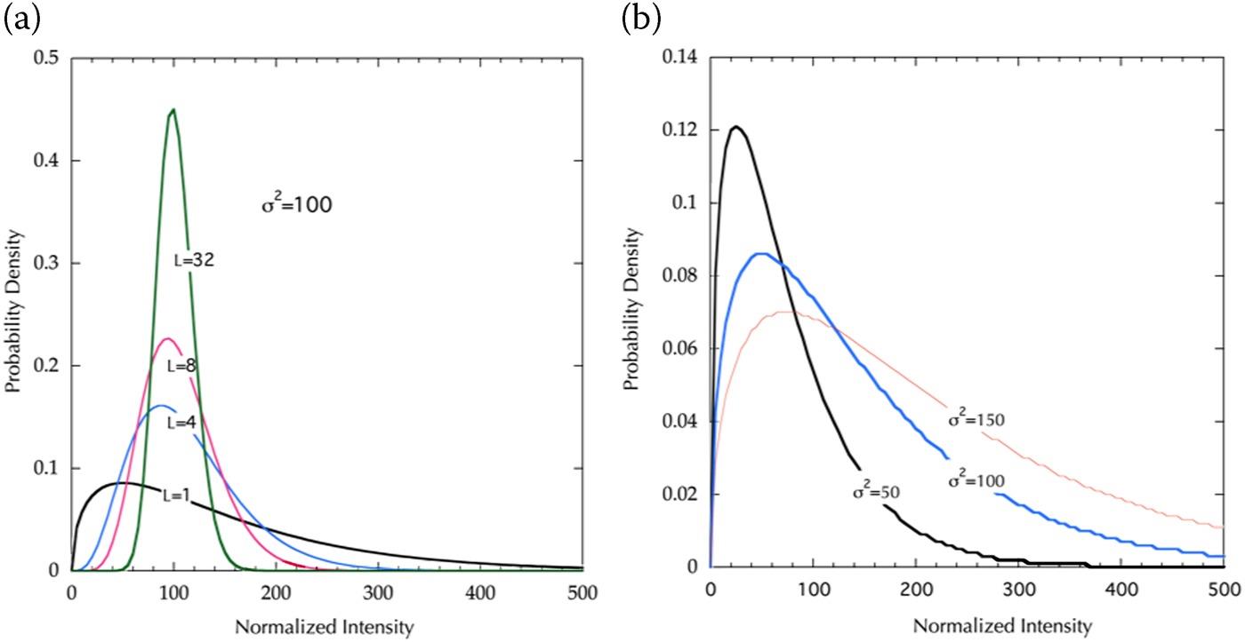
FIGURE 6.1 Amplitude distributions for (a) different look with ; (b) different speckle with L = 1.
For a Gamma distributed speckle, by Bayesian estimation, the L-look amplitude distribution is a K-distribution [4,5]
where is the modified Bessel function of the second kind, ordered ; is an order parameter. Figure 6.2 plots the distributions with values. It is seen that K-distribution has longer tails than Rayleigh distribution. The K-distribution is consistent with a large number of coherent scattering experiments, over wavelengths from optical to sonar, and types of scatterer from atmospheric turbulence to natural radar clutter (both sea and land clutters) [1]. When , the K-distribution approaches to Rayleigh distribution, i.e., tends to be more spatially homogeneous and contains purer speckle.
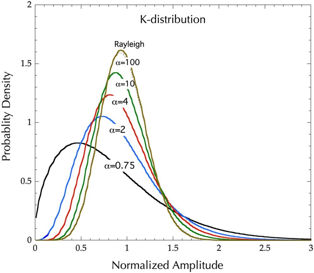
FIGURE 6.2 K-distributions with values of 0.75, 2, 4, 10, and 100. Also included is a Rayleigh distribution.
Notice that the moment of the amplitude in Equation 6.7
Using the preceding formula, we can estimate the order parameter from observed data and test the goodness of fit, which may be done by Kolmogorov–Smirnov (K–S) test [4,5], for example. We also note that the RCS fluctuations are assumed on a much greater spatial scale than speckle so that multi-looking averages speckle without affecting RCS fluctuations.
Now back to Equation 6.3, the value of the speckle strength, , is nothing more than the scattering strength from a rough surface. For remote sensing of soil or sea surface, is the desired quantity to estimate through Equation 6.3 or Equation 6.4. To better infer the surface parameters (roughness, permittivity, etc.), it is a prerequisite to have a good estimate of the scattering coefficients vector from radar measurements. Before proceeds, we note that as an analog to Equation 6.2, the performance measure for the estimated is [6]:
Following the conventional notation in statistical signal processing, let the unknown parameters of interest be , . Then the estimator is any transformation
where is formed by independent samples. As the radar received signal (amplitude) A is a random variable, so is the estimate ; that is, no measurements yield the same values of scattering coefficients. Two criteria are commonly used to obtain the estimate depending on the availability of the probability density function of , .
If the a priori is known, then posteriori is possibly attainable by Bayes’ rule:
The optimal estimate is possible obtained by maximizing the right-hand side of Equation 6.12, and is called maximum a posteriori (MAP) estimator:
Instead of maximizing the probability of a posteriori , we can take the mean value of it, and is called the minimum mean square error (MMSE) estimator:
which yields the estimate with minimum deviation from the true value.
Both MAP and MMSE estimators belong to the Bayesian estimator. For a specific scene to be measured, in general the a priori is unknown or difficult to obtain. In such a case, we may and perhaps have to ignore the a priori . Then we can obtain the estimate simply by maximizing , the so-called maximum likelihood estimator:
For a polarimetric radar, e.g., SAR or scatterometer system, the parameters of interest are the scattering matrix, which can be also multi-frequency, multi-angle, and multi-temporal, etc., as already mentioned above.
6.2 CRAMER–RAO BOUND
In all approaches, the mean square error induced by the estimator is
where is ensemble average over number of measurements; the bias is ; cov is covariance; denote Hermitian transpose operator.
At this point, it is understood that the estimate can be either unbiased or biased. The MSE serves as a performance measure of a parameter’s estimator. The Cramér–Rao bound (CRB) sets the lower value of the covariance for an unbiased estimator with parametric pdf that can be asymptotically attained by the ML estimator for a large number of observations.
Let be the unbiased estimator from the set ; the CRB sets the lower bound of the error covariance:
where is Fisher information matrix and assume positive definite:
The diagonal terms of is the mean square error of the unbiased estimator for with lower bound:
It is seen that for a biased estimator, the minimum square error is larger than CRB.
6.3 LEAST SQUARE ESTIMATION
There are applications where it is necessary to estimate the values of a set of parameters based on the generation model of the deterministic part of the data but without a knowledge of the involved pdfs. In this case one can estimate the parameter values by minimizing the error between the data and the model, according to some metric. A common metric is the sum of the square of the error, and the estimation method is the least-squares (LS) technique. The LS is used in a large variety of applications due to its simplicity in the absence of any statistical model, and for this reason it can be considered an optimization technique for data-fitting rather than an estimation approach. Furthermore, LS has no proof of optimality, except for some special cases where LS coincides with MLE as for additive Gaussian noise, and it is the first pass approach in complex problems.
In radar remote sensing of parameters vector x, it is through a geophysical model function GMF, ;
where , is radar measurement vector, containing the radar scattering coefficients at different channels of measurements by combinations of polarization, angular, frequency, temporal, or spatial diversities, including angular and frequency correlations. Here the radar scattering coefficients are not limited by backscattering only, as was done traditionally.
In general, is a complex and highly nonlinear function that relates the input vector (observation space) and the output vector (parameter space) includes an electromagnetic scattering model, dielectric model (e.g., soil and ocean surface), and wind-wave model (ocean), where the electromagnetic scattering model describes the relationship between the radar echo and the target parameters (both geometrical and electrical), while the dielectric model or the wind-wave model converts the electrical parameters to the physical parameters of interest (e.g., soil moisture content, ocean winds). Reminding from the uncertainties of the roughness parameters, and RCS measurements in previous chapters, what we discussed about (6.1) is an ideal case. In practice, uncertainties must, more or less, be attached to , , and . Physically, the noise sources come from different aspects. For roughness parameters, please refer to Equations 2.40 and 2.41 in Chapter 2.
A data model, in a proper way, is to enable a mapping of measurement space to parameter space, which we are of interest. Here, following, we detail the procedures. To be more explicitly and realistic, Equation 6.20 is re-expressed by
where is the surface parameters vector; matrix relates the surface parameters vector to radar scattering measurements , and represents the measurement error vector induced by system and calibration errors, and speckle noise. Note that the radar response is formed by, in general, the scattering matrix. Knowing that small values for or will result in a more accurate estimate and that both and are random variables, we now deal with the mapping between x and y. That is, we need to find a good estimator for from . Building the relationship between and , both experimental and theoretical methods may be applied, but both will introduce the issues of resolution, distortion, fuzziness and noise. This, equivalently, requires a function, . In practice, we are never able to get a noise-free inverse function . An approximate , in statistical or deterministic form, is usually applied.
From previous discussions, we may summarize the estimation error sources in terms of the remote sensing of surfaces as (1) the surface parameter uncertainty and (2) the measurement uncertainty, as described in Equation 6.21. Fur one often faces the situation where one measurement set must be mapped to more than one parameter set; i.e., an ill-posed problem. As shown in Figure 6.3 the parameter sets (object domain) correspond to the same measurement result (data domain). If we want to determine one representative value , in the minimum squared error sense, a sample average of the known parameter sets will be used as the retrieval result. As in mapping problem, there always come with issues of uniqueness, existence, and stability. Regularization theory and neural networks with deep learning are often applied to resolve these problematic issues.
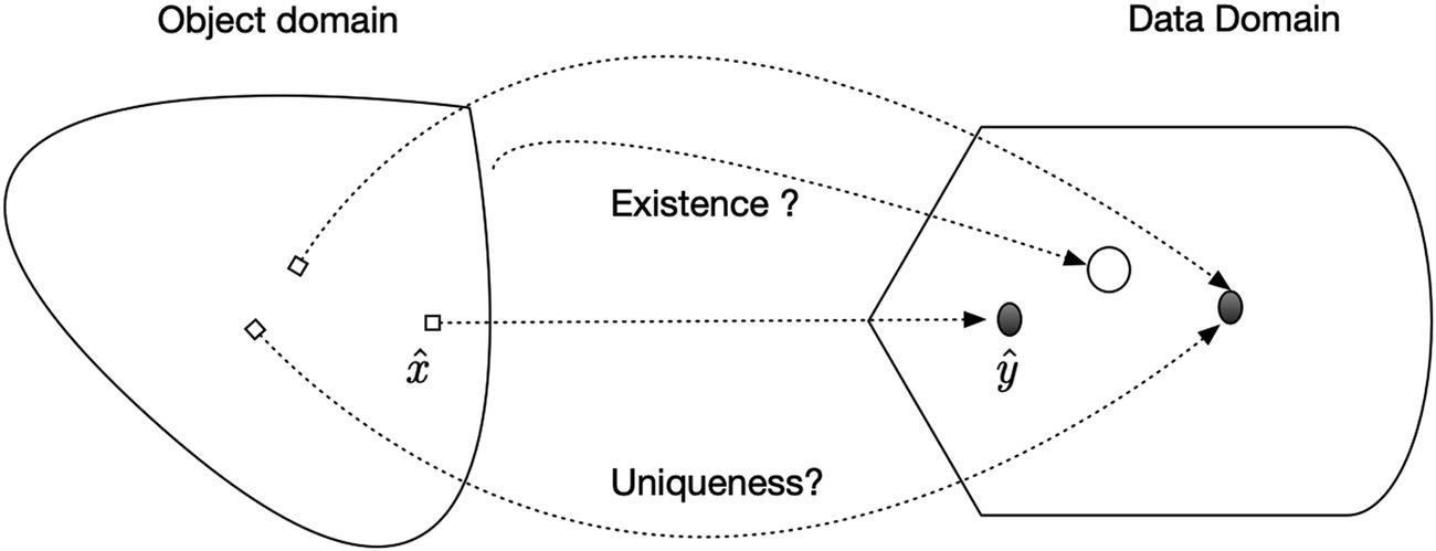
FIGURE 6.3 Mapping of parameters from measurements.
6.4 KALMAN FILTER-BASED ESTIMATION
It has been illustrated from previous chapters, the inverse mapping from radar measurements to surface parameters will be highly nonlinear and an analytic function does not usually exist. Indeed, the retrieval of surface parameters can be viewed as a problem of mappings from the measured signal domain onto the range of surface characteristics that quantify the observation [7–9]. To solve the problems of multidimensional retrieval, the application of a neural network to microwave remote sensing has been carried out by many investigators, because of its ability to adapt to geophysical multidimensionality and its noise robustness in realistic remote sensing. It becomes apparent that the parameter estimation problem invokes two issues that must be simultaneously solved. One is the need for an inversion scheme that provides the mapping, between the parameters to be inferred and the measurements, in a least-squares error sense. Because parameter estimation must come from a finite set of radar observations and measurements, an ill-posed must be solved. Neural networks seem to be well suited for these purposes. Another is the need for GMF models that relate the radar echoes and the geophysical parameters. Thus, the GMF includes two parts: the scattering model relating to the dependence of radar returns to surface roughness and permittivity; the dielectric model relating the permittivity to the moisture content under various conditions.
The Kalman filter (KF) is the optimal MMSE estimate of the state for time-varying linear systems and Gaussian processes in which the evolution of the state is described by a linear dynamic system. In a statistical sense, constitutes a random variable due to spatially and temporally varying properties, such that
where is true variable, and is noise term.
In practice, the “truth” is never obtainable; it is always vague. Statistically, and may be assumed to be, as they usually are, uncorrelated, such that is an unbiased estimate of , i.e.,
where E denotes statistical mean, is variance of .
Note that the radar response is formed by, in general, the scattering matrix. It has been argued that [10] non-quadratic regularization is practically effective in minimizing the clutter while enhancing the target features via:
where denotes (), and is a scalar parameter and is recognized as the cost or objective function.
Direct solving of Equation 6.24 perhaps is possible but demands intensive computation resources. From preceding chapters, we also see that the scattering behavior, both pattern and strength is complicatedly determined, in a stochastic sense, by three surface parameters. Hence, in search of the cost function minima in Equation 6.24, we may seek a neural network approach. Perhaps one disadvantage of the neural network is that it constitutes a black box for most users. Extensive studies show that it is a powerful tool for handling complex problems involving bulky volume data in high dimensional feature space. The inverting parameters vector from measurements, a neural network offers an effective and efficient approach and will be detailed in what follows.
Modified from a multilayer perceptron (MLP), a dynamic learning neural network (DLNN) was proposed [11] and is adopted. Figure 6.4 schematically depicts the configuration of a dynamic learning neural network (DLNN). It features: (1) every node at the input layer and all hidden layers are fully connected to the output layer; (2) the activation function is removed from each output node; the output of the modified network can be characterized as the weighted sum of the polynomial basis vectors. Such modifications form a condensed model of the MLP in which the output is a weighted sum of compositions of polynomials. Hence, with measurement error matrix , as in Equation 6.1, is the network weight matrix.
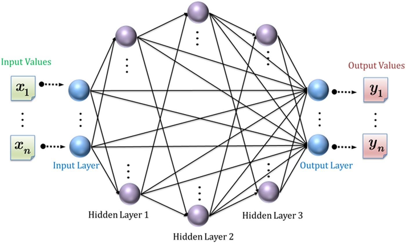
FIGURE 6.4 Network structure of a dynamic learning neural network (DLNN). It features every node at input layer and all hidden layers are fully connected to the output layer; the activation function is removed from each output node; the output of the modified network can be characterized as the weighted sum of the polynomial basis vectors.
The network training or learning scheme, based on the Kalman filter technique [12] that lends itself to a highly dynamic and adaptive merit during the learning stage, is described below. To begin, the basic concept of Kalman filtering is briefly described, with notation given in Figure 6.5.
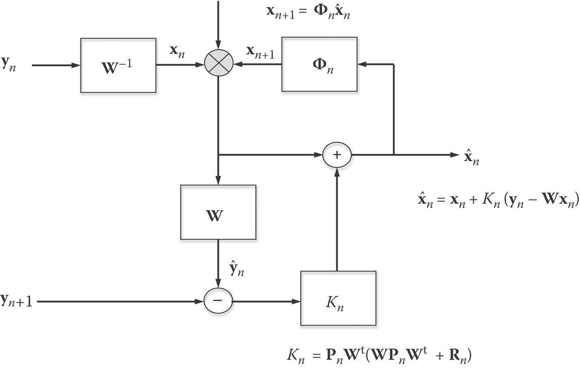
FIGURE 6.5 Schematic description of Kalman filtering.
The measurement equation takes the form for one-step n:
where the subscript n denotes the measurement at a discrete nth time step. The process equation relates to the transition states of the surface parameters vector x:
where is a transition matrix, is the process error vector, and is the error matrix which, in our case, is a diagonal matrix.
The measurement error and process error may be assumed to be statistically independent, i.e.,
where is the one-step predicted estimate, is the filter estimate of the desired and is the computed Kalman gain. For numerical stability, its computation takes the following steps:
where are the one-step predicted and filter estimate error covariance matrices, respectively. The initial state can be set as .
For the error vectors, it is physically reasonable to assume that for both measurement and process error vectors:
where are error covariance matrices, respectively. The process error and the measurement error in radar observation may be reasonably assumed to be statistically independent and can be modeled as zero-mean, white noise process.
From the modified MLP structure, each updated estimate of the neural network weight is computed from the previous estimate and the new input data. The weights connected to each output node can be updated independently such that the vector problem can, therefore, be decomposed into scalar problems as
Applying to the Kalman filtering technique, the network structure can be modeled by
where the superscript denotes the training pattern with total of N, is a by state transition matrix, is a by diagonal matrix, represents a 1 by process error vector, with M the dimension of concatenated activations in modified MLP, and is a scalar measurement error.
The update of network weights is according to the following recursions:
where is the desired output, is the one-step predicted estimate, and is the filter estimate of , respectively, and is the computed Kalman gain, which is viewed as an adaptive learning rate and its computation is according to Equations 6.31–6.35.
From the previous chapter, the sensitivity analysis in response to radar scattering is essential. Knowing the parameter bounds is important to the network performance. A neural-based estimation seems powerful and yet efficient as long as training data is effective. The MLP together with learning by Kalman filter is expected to resolve the highly nonlinear, and complex decision boundary problems, as will be demonstrated in the following chapter.
References
1. Lee, J. S., and Pottier, E., Polarimetric Radar Imaging—From Basics to Applications, CRC Press, Boca Raton, FL, 2009.
2. Chen, K. S., Wu, T. D., and Shi, J. C., A model-based inversion of rough soil surface parameters from radar measurements, Journal of Electromagnetic Waves and Applications, 15(2), 173–200, 2001.
3. Ulaby, F. T., Moore, R. K., and Fung, A. K., Microwave Remote Sensing, Addison-Wesley, Reading, MA, 1982.
4. Lehmann, E. L., and Romano, J. P., Testing Statistical Hypotheses, 3rd edn Edition, Springer, New York, 2005.
5. Spagnolini, U., Statistical Signal Processing in Engineering, John Wiley & Sons, New York, 2018.
6. Long, D. G., and Spencer, M. W., Radar backscatter measurement accuracy for a spaceborne pencil-beam wind scatterometer with transmit modulation, IEEE Transactions on Geoscience and Remote Sensing, 35(17), 102–114, 1997.
7. Chen, K. S., Kao, W. L., and Tzeng, Y. C., Retrieval of surface parameters using dynamic learning neural network, International Journal of Remote Sensing, 16, 801–809, 1995.
8. Thiria, S., Mejia, C., and Badran, F., A neural network approach for modeling nonlinear transfer functions: Application for wind retrieval from space borne scatter meter data, Journal of Geophysical Research: Oceans, 98, 22827–22841, 1993.
9. Chen, K. S., Tzeng, Y. C., and Chen, P. C., Retrieval of ocean winds from satellite scatter meter by a neural network. IEEE Transactions on Geoscience and Remote Sensing, 37, 247–256, 1999.
10. Çetin, M., and Karl, W. C., Feature-enhanced synthetic aperture radar image formation based on nonquadratic regularization. IEEE Transactions on Image Processing, 10, 623–631, 2001.
11. Tzeng, Y. C., Chen, K. S., Kao, W. L., and Fung, A. K., A dynamic learning neural network for remote sensing applications. IEEE Transactions on Geoscience and Remote Sensing, 32, 1096–1102, 1994.
12. Scharf, L. L., Statistical Signal Processing—Detection, Estimation, and Time-Series Analysis, Addison Wesley Publishing Co., Reading, MA, 1991.