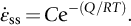
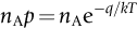
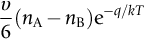
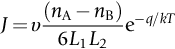
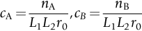
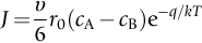
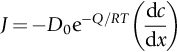
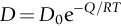
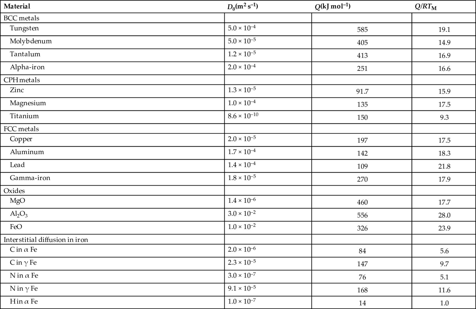
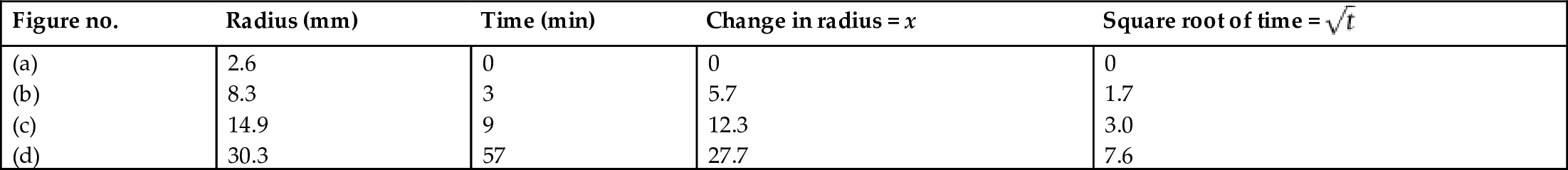
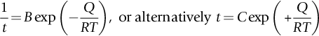
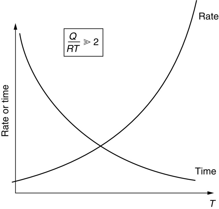
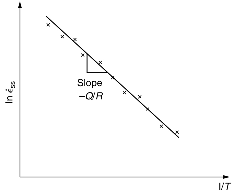
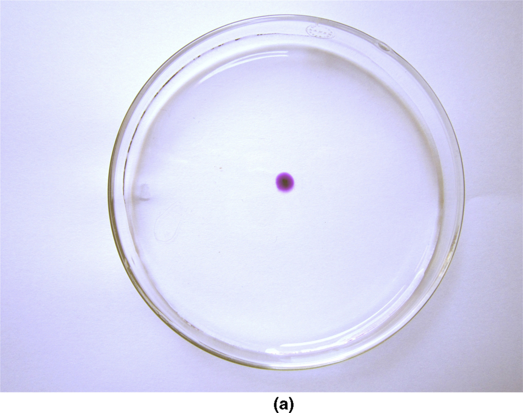
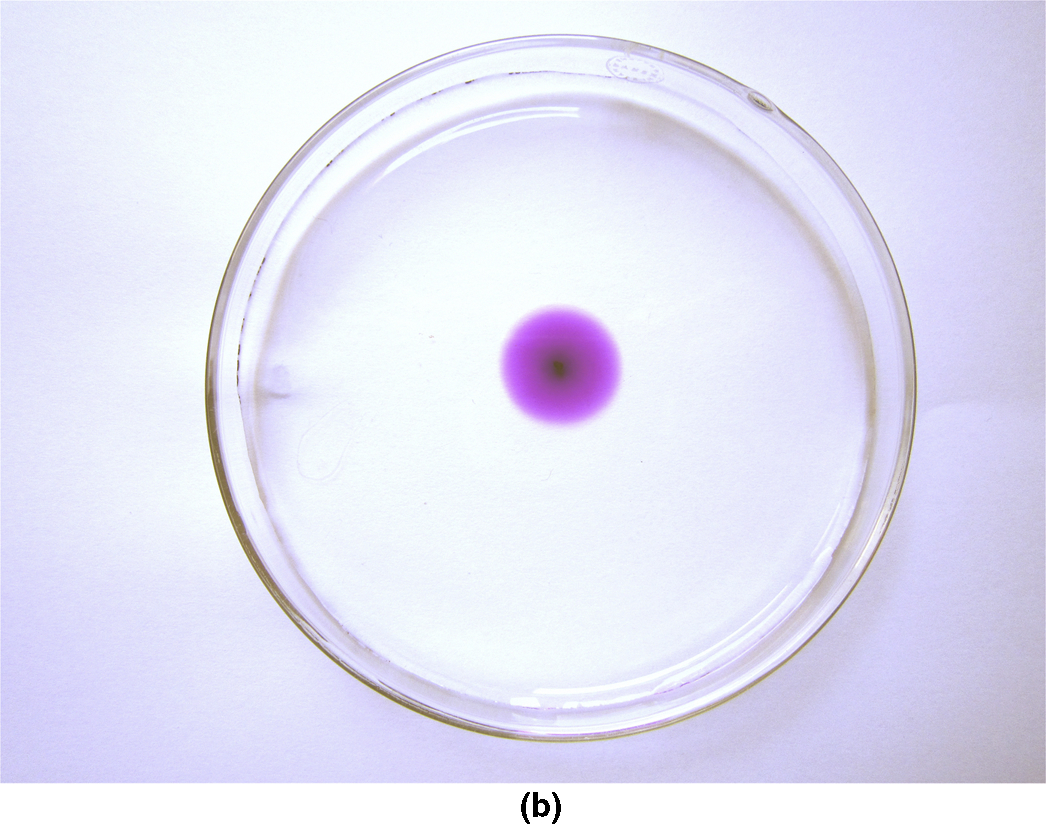
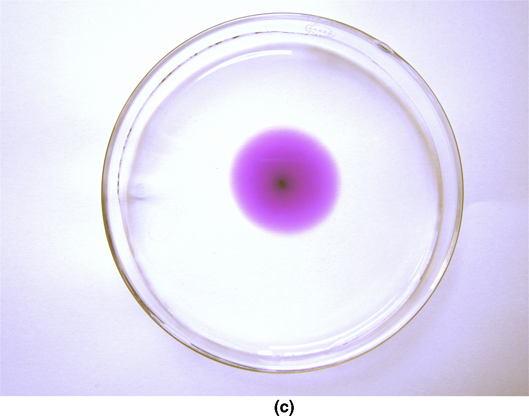
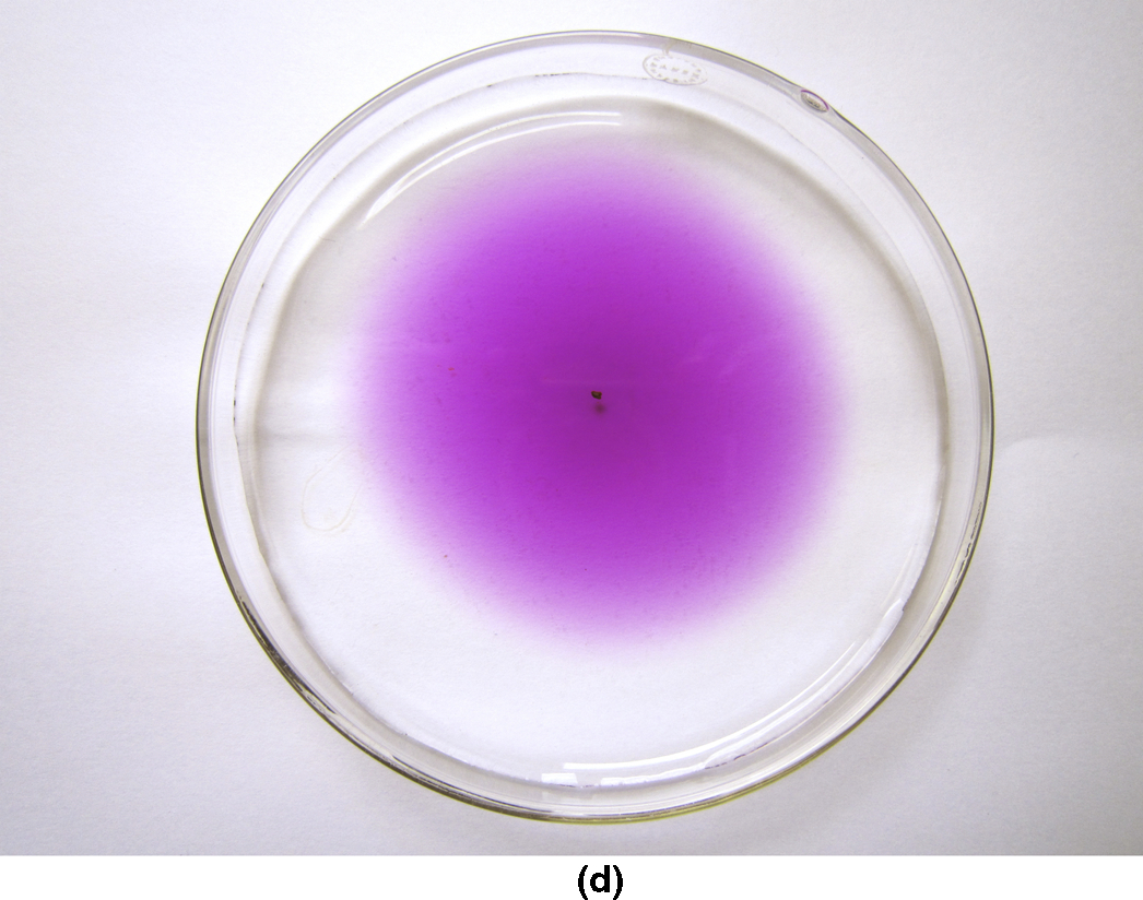
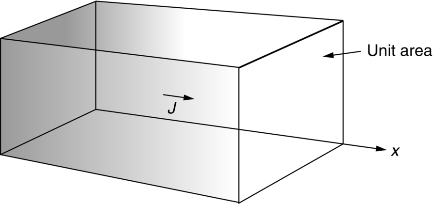
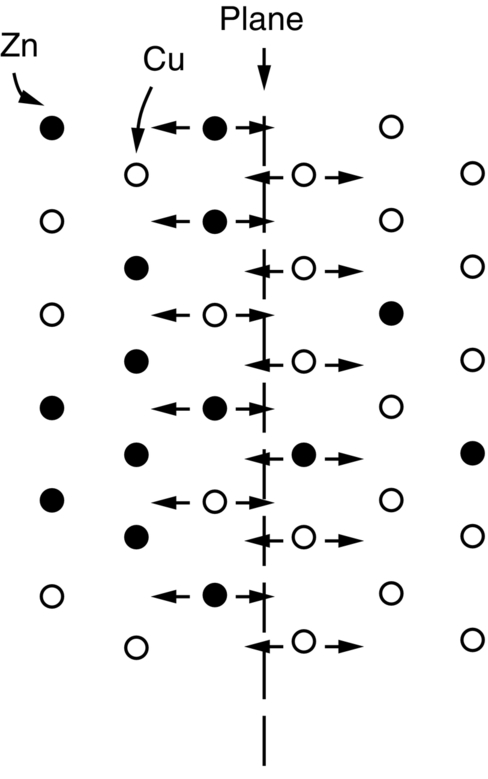
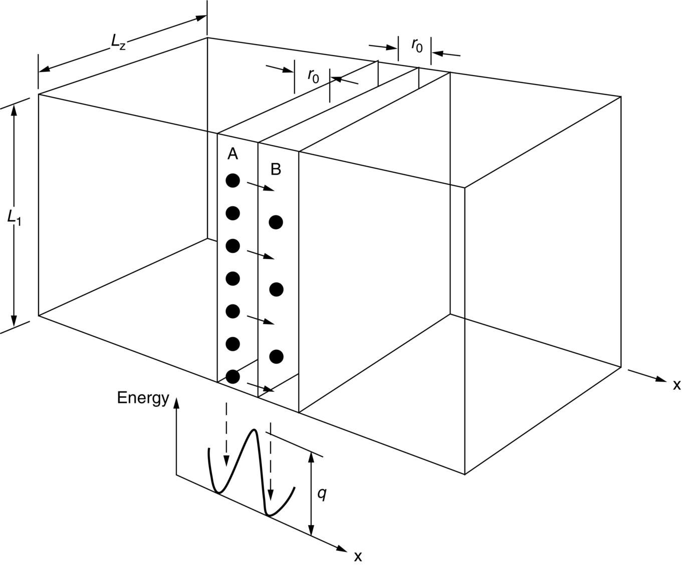
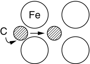
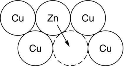
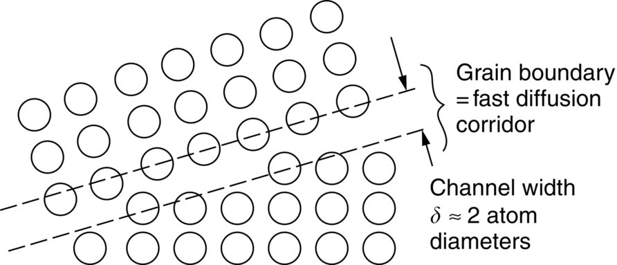
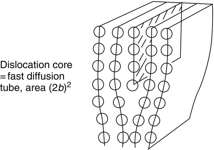
section epub:type=”chapter”> This chapter discusses the kinetic theory of diffusion. The rate of steady-state creep varies with temperature. έss = Ce-(Q/ṜT). This is an example of Arrhenius’s law. Like all good laws, it has great generality. Thus, it applies not only to the rate of creep, but also to the rate of oxidation, the rate of corrosion, the rate of diffusion, even to the rate at which bacteria multiply and milk turns sour. The chapter states that the rate of the process (creep, corrosion, diffusion, etc.) increases exponentially with temperature (or, equivalently, that the time for a given amount of creep, or of oxidation, decreases exponentially with temperature). If the rate of a process that follows Arrhenius’s law is plotted on a loge scale against 1/T, a straight line with a slope of –Q/Ṝ is obtained. The value of Q characterizes the process. The chapter discusses the origin of Arrhenius’s law and its application to diffusion. This is followed by the discussion of diffusion and Fick’s law and data for diffusion coefficients. The chapter concludes with a discussion of mechanisms of diffusion. We saw in the last chapter that the rate of steady-state creep, Here Q is the activation energy for creep (J mol–1), R is the universal gas constant (8.31 J mol–1 K–1) and T is the absolute temperature (K). This is an example of Arrhenius’s law. Like all good laws, it has great generality. Thus it applies not only to the rate of creep, but also to the rate of oxidation (Chapter 25), the rate of corrosion (Chapter 27), the rate of diffusion (this chapter), even to the rate at which bacteria multiply and milk turns sour. It states that the rate of the process (creep, corrosion, diffusion, etc.) increases exponentially with temperature (or, equivalently, that the time for a given amount of creep, or of oxidation, decreases exponentially with temperature) in the way shown in Figure 22.1. If the rate of a process that follows Arrhenius’s law is plotted on a loge scale against 1/T, a straight line with a slope of In this chapter, we discuss the origin of Arrhenius’s law and its application to diffusion. In the next, we examine how it is that the rate of diffusion determines that of creep. First, what do we mean by diffusion? A good way of demonstrating it is to take a glass Petri dish, and run a very shallow layer of water into it. Wait until the water is totally still, and then drop a very small crystal of potassium permanganate into it. The edge of the crystal will immediately begin to dissolve in the water, producing a dark pink ring of solution centered on the crystal—see Figure 22.3(a). The ring then begins to spread radially outward into the layer of water—initially very quickly, but progressively more slowly as time passes. Figures 22.3(a) to 22.3(d) are time-lapse photographs showing the ring spreading. This is caused by the movement of potassium permanganate ions by random exchanges with the water molecules. The ions move from regions where they are concentrated to regions where they are less concentrated—the ions diffuse down the concentration gradient. This behavior is described by Fick’s first law of diffusion: J is the number of ions diffusing down the concentration gradient per second per unit area; it is called the flux of ions (Figure 22.4). c is the concentration of ions in the water—the number of ions (in this case permanganate ions) per unit volume of solution. x is the distance measured along the flux lines, and D is the diffusion coefficient for permanganate ions in solution—it has units of m2 s–1. This diffusive behavior is not just limited to ions in water—it occurs in all liquids, and more remarkably, in all solids as well. As an example, in the alloy brass—a mixture of zinc in copper—zinc atoms diffuse through the solid copper in just the way that ions diffuse through water. Because the materials of engineering are mostly solids, we shall now confine ourselves to talking about diffusion in the solid state. Physically, diffusion occurs because atoms, even in a solid, are able to move—to jump from one atomic site to another. Figure 22.5 shows a solid in which there is a concentration gradient of black atoms: there are more to the left of the broken line than there are to the right. If atoms jump across the broken line at random, then there will be a net flux of black atoms to the right (simply because there are more on the left to jump), and, of course, a net flux of white atoms to the left. Fick’s law describes this. It is derived in the following way. The atoms in a solid vibrate, or oscillate, about their mean positions, with a frequency υ (typically about 1013 s–1). The crystal lattice defines these mean positions. At a temperature T, the average energy (kinetic plus potential) of a vibrating atom is 3kT where k is Boltzmann’s constant (1.38 × 10⁻²³ J atom–1 K–1). But this is only the average energy. As atoms (or molecules) vibrate, they collide, and energy is continually transferred from one to another. Although the average energy is 3kT, at any instant, there is a certain probability that an atom has more or less than this. A very small fraction of the atoms have, at a given instant, much more—enough, in fact, to jump to a neighboring atom site. It can be shown from statistical mechanical theory that the probability, p, that an atom will have, at any instant, an energy Why is this relevant to the diffusion of zinc in copper? Imagine two adjacent lattice planes in the brass with two slightly different zinc concentrations, as shown in exaggerated form in Figure 22.6. Let us denote these two planes as A and B. Now for a zinc atom to diffuse from A to B, down the concentration gradient, it has to “squeeze” between the copper atoms (a simplified statement—but we shall elaborate on it in a moment). This is another way of saying: the zinc atom has to overcome an energy barrier of height q, as shown in Figure 22.6. Now, the number of zinc atoms in layer A is nA, so the number of zinc atoms that have enough energy to climb over the barrier from A to B at any instant is For these atoms actually to climb over the barrier from A to B, they must of course be moving in the correct direction. The number of times each zinc atom oscillates toward B is ≈ υ/6 s–1 (there are six possible directions in which the zinc atoms can move in three dimensions, only one of which is from A to B). Thus the number of atoms that actually jump from A to B per second is But, meanwhile, some zinc atoms jump back. If the number of zinc atoms in layer B is nB, the number of zinc atoms that can climb over the barrier from B to A per second is Thus the net number of zinc atoms climbing over the barrier per second is The area of the surface across which they jump is L1L2, so the net flux of atoms, using the definition given earlier, is: Concentrations, c, are related to numbers, n, by where cA and cB are the zinc concentrations at A and B and r0 is the atom size. Substituting for nA and nB in Equation (22.8) gives But, (cA – cB)/r0 is the concentration gradient, dc/dx. The quantity q is inconveniently small and it is better to use the larger quantities Q = NAq and R = NAk, where NA, is Avogadro’s number. The quantity and this is just Fick’s law (Equation 22.2) with This method of writing D emphasizes its exponential dependence on temperature, and gives a conveniently sized activation energy (expressed per mole of diffusing atoms rather than per atom). Thinking again of creep, the thing about Equation (22.12) is that the exponential dependence of D on temperature has exactly the same form as the dependence of Diffusion coefficients are best measured in the following way. A thin layer of a radioactive isotope of the diffusing atoms or molecules is plated onto the bulk material (e.g., radioactive zinc onto copper). The temperature is raised to the diffusion temperature for a measured time, during which the isotope diffuses into the bulk. The sample is cooled and sectioned, and the concentration of isotope measured as a function of depth by measuring the radiation it emits. D0 and Q are calculated from the diffusion profile. Materials handbooks list data for D0 and Q for various atoms diffusing in metals and ceramics—Table 22.1 gives some useful values. Diffusion occurs in polymers, composites, and glasses, too, but the data are less reliable. The last column of the table shows the normalized activation energy, Q/RTM, where TM is the melting point (in degrees kelvin). It has been found that, for a given class of material (e.g., f.c.c. metals, or refractory oxides), the diffusion parameter D0 for mass transport—the one that is important in creep—is roughly constant; and the activation energy is proportional to the melting temperature TM (K) so Q/RTM, too, is a constant (which is why creep is related to the melting point). This means that many diffusion problems can be solved approximately using the data given in Table 22.2, which shows the average values of D0 and Q/RTM, for material classes. Table 22.2 In our discussion so far we have sidestepped the question of how the atoms in a solid move around when they diffuse. There are several ways in which this can happen. For simplicity, we shall talk only about crystalline solids, although diffusion occurs in amorphous solids as well, and in similar ways. Diffusion in the bulk of a crystal can occur by two mechanisms. The first is interstitial diffusion. Atoms in all crystals have spaces, or interstices, between them, and small atoms dissolved in the crystal can diffuse by squeezing between atoms, jumping—when they have enough energy—from one interstice to another (Figure 22.7). Carbon, a small atom, diffuses through steel in this way; in fact C, O, N, B, and H diffuse interstitially in most crystals. These small atoms diffuse very quickly. This is reflected in their very small values of Q/RTM, seen in the last column of Table 22.1. The second mechanism is that of vacancy diffusion. When zinc diffuses in brass, for example, the zinc atom (comparable in size to the copper atom) cannot fit into the interstices—the zinc atom has to wait until a vacancy, or missing atom, appears next to it before it can move. This is the mechanism by which most diffusion in crystals takes place (Figures 22.8 and 11.4). Diffusion in the bulk crystals may sometimes be short circuited by diffusion down grain boundaries or dislocation cores. The boundary acts as a planar channel, about two atoms wide, with a local diffusion rate which can be as much as 106 times greater than in the bulk (Figures 22.9 and 11.4). The dislocation core, too, can act as a high conductivity “wire” of cross-section about (2b)2, where b is the atom size (Figure 22.10). Of course, their contribution to the total diffusive flux depends also on how many grain boundaries or dislocations there are: when grains are small or dislocations numerous, their contribution becomes important. Because the diffusion coefficient D has units of m2 s–1, is a useful result for estimating diffusion distances in a wide range of situations. The demonstration of diffusion shown in Figure 22.3 can be used to verify Equation (22.13) and also give us an estimate of the diffusion coefficient. The Following Table gives the data. The plot of x against
Kinetic Theory of Diffusion
Publisher Summary
22.1 Introduction
 , varies with temperature as
 is obtained (Figure 22.2). The value of Q characterizes the process—a feature we have already used in Chapter 21.
22.2 Diffusion and Fick’s Law
 is
is
 /6 is usually written as D0. Making these changes gives:
 on temperature that we seek to explain.
22.3 Data for Diffusion Coefficients
Material Class
D0(m2 s–1)
Q/RTM
BCC metals (W, Mo, Fe below 911°C, etc.)
1.6 × 10⁻⁴
17.8
CPH metals (Zn, Mg, Ti, etc.)
5 × 10⁻⁵
17.3
FCC metals (Cu, Al, Ni, Fe above 911°C, etc.)
5 × 10⁻⁵
18.4
Alkali halides (NaCl, LiF, etc.)
2.5 × 10⁻³
22.5
Oxides (MgO, FeO, Al2O3, etc.)
3.8 × 10⁻⁴
23.4
22.4 Mechanisms of Diffusion
Bulk diffusion: Interstitial and vacancy diffusion
Fast diffusion paths: Grain boundary and dislocation core diffusion
A useful approximation
 has units of meters. The length scale of
  is in fact a good approximation to the distance that atoms diffuse over a period of time t. The proof of this result involves nonsteady diffusion (Fick’s second law of diffusion) and we will not go through it here. However, the approximation
Worked example
 is a pretty good straight line, consistent with Equation (22.13). The value of D can also be estimated because the slope of the plot
  .
.
Examples
 , calculate how long the process will take at 227°C.
where R is the universal gas constant and T is the absolute temperature. The constants D0 and Q have the values 9.5 mm2 s−1 and 159 kJ mol−1, respectively.
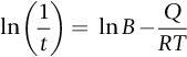
Answers
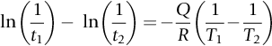
As in Example 21.2, use the natural log (ln) form of this equation
then write it out twice, and subtract
to give Q = 8.0 × 10⁴ J mol−1. Remember to input temperatures in units of K. Putting this value of B into the initial equation for either pair of t, T gives B = 6.4 × 10⁷ s−1. Finally, input T3 = 500 K into the initial equation with the values of Q and B already determined, to give t3 = 3.6 s.