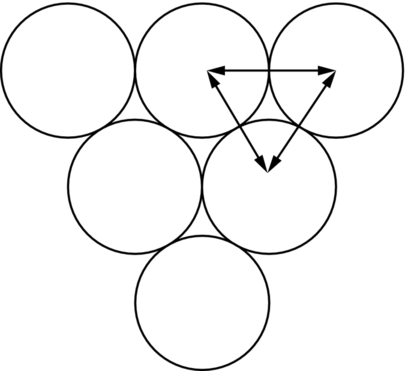
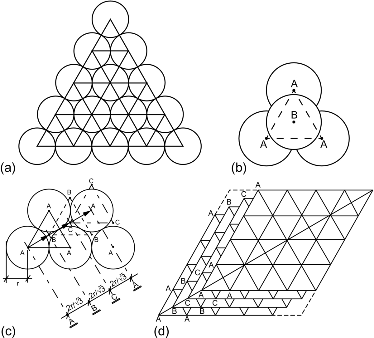
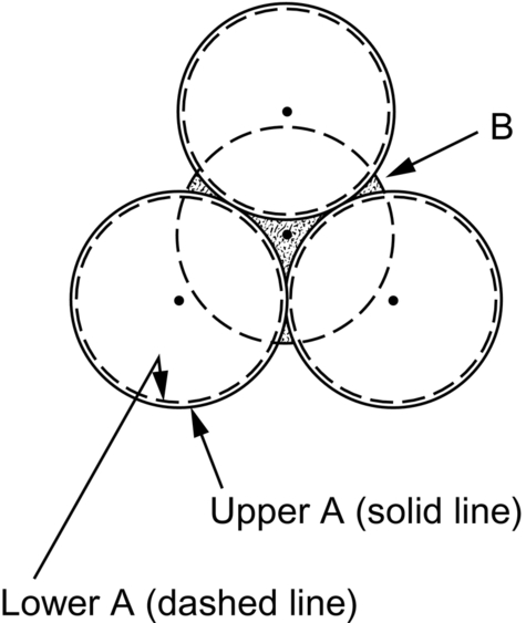
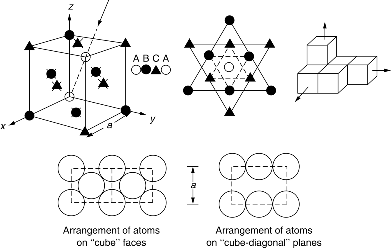
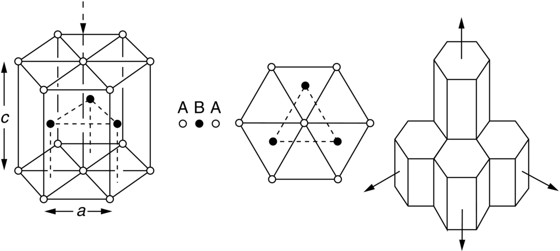
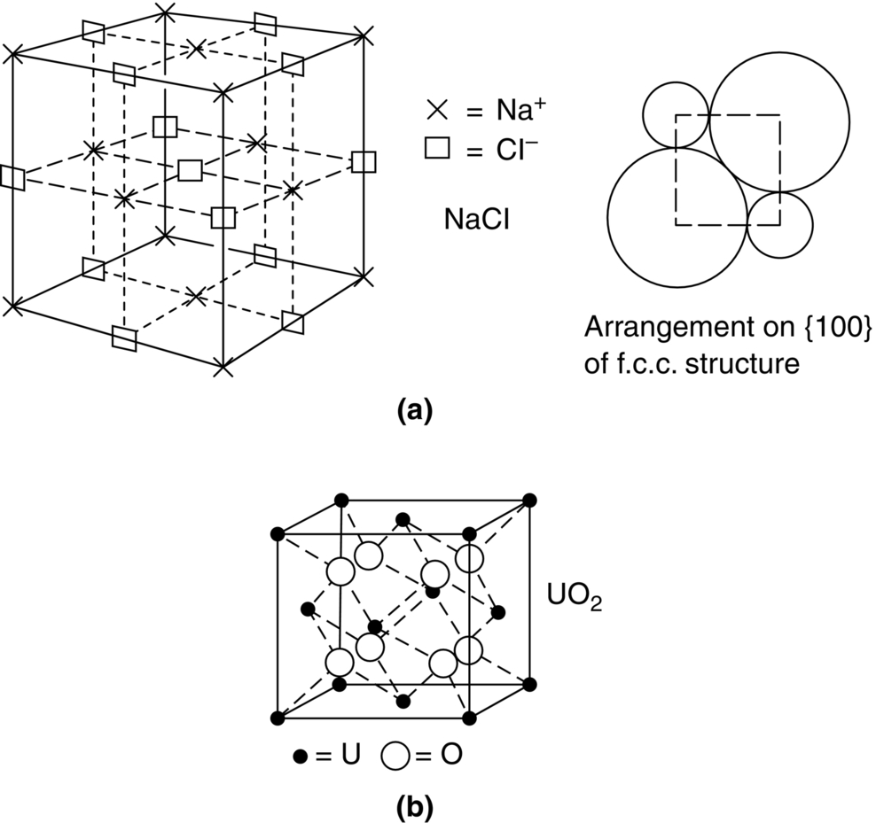
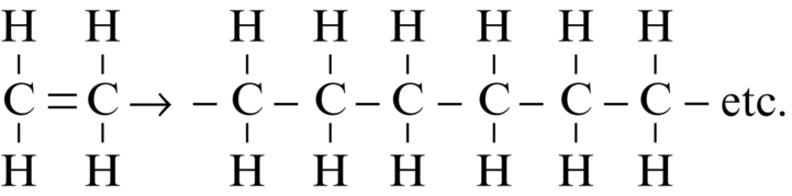
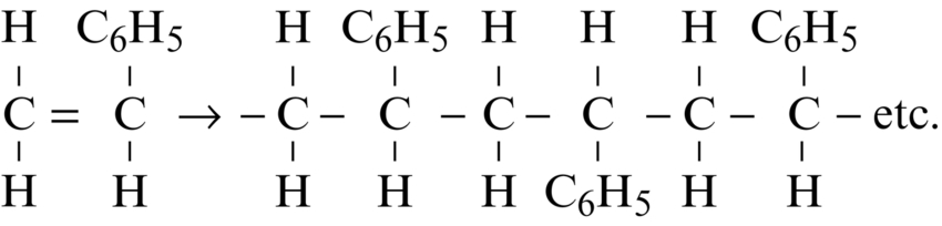
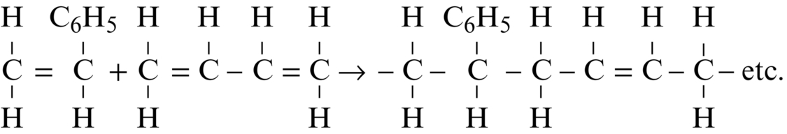
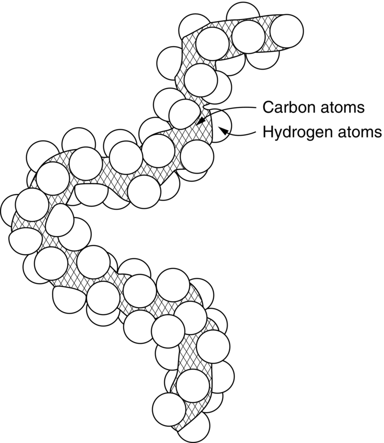
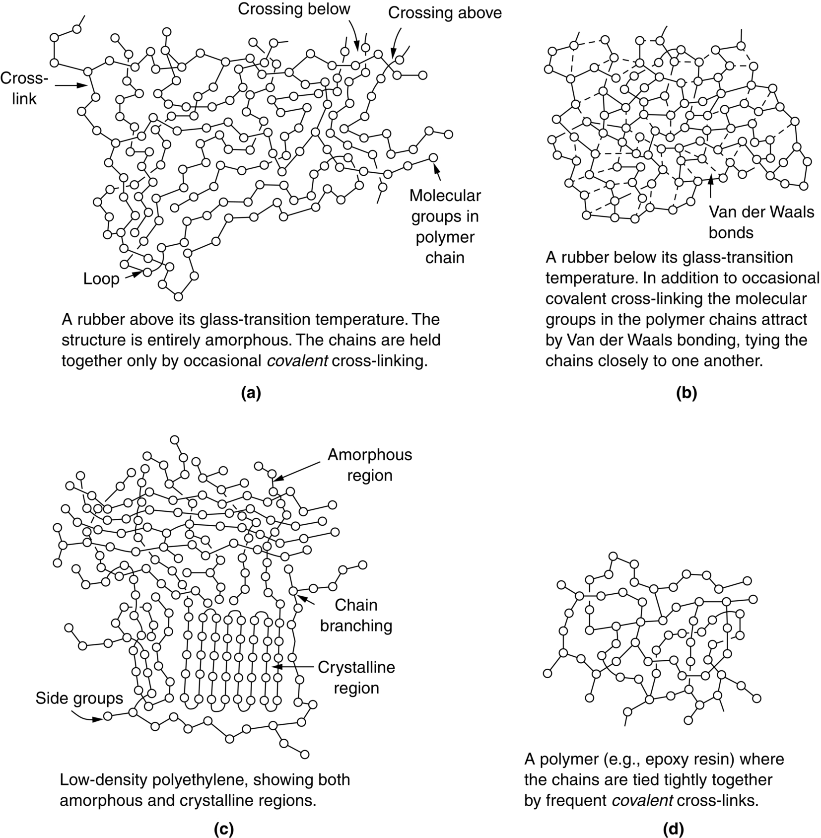
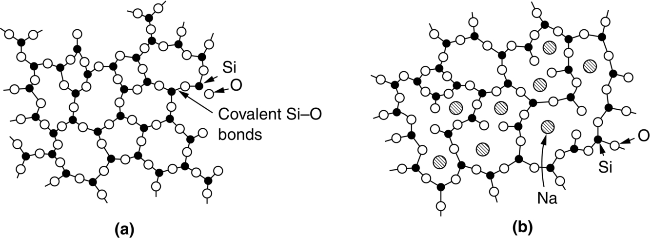
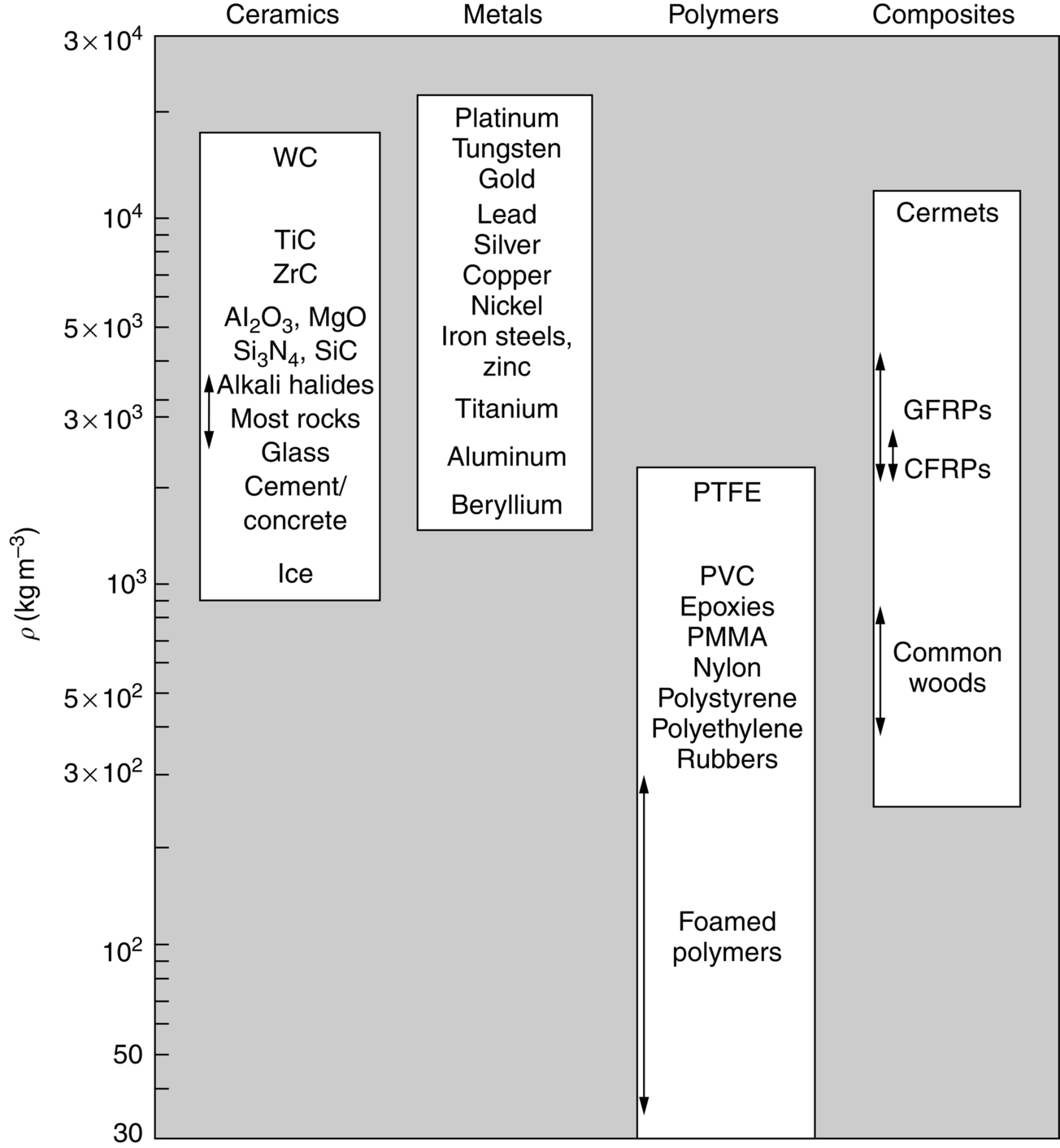
section epub:type=”chapter”> This chapter examines how atoms are arranged in main engineering solids. Many engineering materials (almost all metals and ceramics, for instance) are made up entirely of small crystals or grains in which atoms are packed in regular, repeating, three-dimensional patterns; the grains are stuck together meeting at grain boundaries. This chapter focuses on the individual crystals that can be best understood by thinking of the atoms as hard spheres. The chapter also discusses close-packed structures and crystal energies followed by crystallography, plane indices, and direction indices. The chapter concludes with a discussion of atom packing in polymers, atom packing in inorganic glasses, and the density of solids. In the previous chapter we examined the stiffnesses of the bonds holding atoms together. But bond stiffness alone does not explain the stiffness of solids; the way in which the atoms are packed together is equally important. In this chapter we examine how atoms are arranged in the main engineering solids. Many engineering materials (almost all metals and ceramics, for instance) are made up entirely of small crystals or grains in which atoms are packed in regular, repeating, three-dimensional patterns; the grains are stuck together, meeting at grain boundaries, which we will describe later. We focus now on the individual crystals, which can best be understood by thinking of the atoms as hard spheres (although, from what we said in the previous chapter, it is clear that this is a simplification). To make things even simpler, for the moment consider a material that is pure—with only one size of hard sphere—which has nondirectional bonding, so we can arrange the spheres subject only to geometrical constraints. Pure copper is a good example of a material satisfying these conditions. To build up a three-dimensional packing pattern, it is easier conceptually to begin by An example of how we might pack atoms in a plane is shown in Figure 5.1; it is the arrangement in which the reds are set up on a billiard table before starting a game of snooker. The balls are packed in a triangular fashion so as to take up the least possible space on the table. This type of plane is thus called a close-packed plane, and contains three close-packed directions; they are the directions along which the balls touch. The figure shows only a small region of close-packed plane—if we had more reds we could extend the plane sideways and could, if we wished, fill the whole billiard table. The important thing to notice is the way in which the balls are packed in a regularly repeating two-dimensional pattern. How could we add a second layer of atoms to our close-packed plane? As Figure 5.1 shows, the depressions where the atoms meet are ideal “seats” for the next layer of atoms. By dropping atoms into alternate seats, we can generate a second close-packed plane lying on top of the original one and having an identical packing pattern. Then a third layer can be added, and a fourth, and so on until we have made a sizeable piece of crystal—with, this time, a regularly repeating pattern of atoms in three dimensions. The particular structure we have produced is one in which the atoms take up the least volume and is therefore called a close-packed structure. The atoms in many solid metals are packed in this way. There is a complication to this apparently simple story. There are two alternative and different sequences in which we can stack the close-packed planes on top of one another. If we follow the stacking sequence in Figure 5.1 rather more closely, we see that, by the time we have reached the fourth atomic plane, we are placing the atoms directly above the original atoms (although, naturally, separated from them by the two interleaving planes of atoms). We then carry on adding atoms as before, generating an ABCABC… sequence. In Figure 5.2 we show the alternative way of stacking, in which the atoms in the third plane are now directly above those in the first layer. This gives an ABAB … sequence. These two different stacking sequences give two different three-dimensional packing structures—face-centered cubic (f.c.c.) and close–packed hexagonal (c.p.h.) respectively. Many common metals (e.g., Al, Cu and Ni) have the f.c.c. structure and many others (e.g., Mg, Zn, and Ti) have the c.p.h. structure. Why should Al choose to be f.c.c. while Mg chooses to be c.p.h.? The answer to this is that materials choose the crystal structure that gives minimum energy. This structure may not necessarily be close packed or, indeed, very simple geometrically—although to be a crystal it must still have some sort of three–dimensional repeating pattern. The difference in energy between alternative structures is often slight. Because of this, the crystal structure that gives the minimum energy at one temperature may not do so at another. Thus tin changes its crystal structure if it is cooled enough; and, incidentally, becomes much more brittle in the process (it is said this caused the tin-alloy coat buttons of Napoleon’s army to fall apart during the harsh Russian winter, and the soldered cans of paraffin on Scott’s South Pole expedition to leak). Cobalt changes its structure at 450ºC, transforming from a c.p.h. structure at lower temperatures to an f.c.c. structure at higher temperatures. More important, pure iron transforms from a b.c.c. structure (defined in the following) to one that is f.c.c. at 911ºC, a process which is important in the heat treatment of steels. We have not yet explained why an ABCABC sequence is called “f.c.c.” or why an ABAB sequence is referred to as “c.p.h.” And we have not even begun to describe the features of the more complicated crystal structures like those of ceramics such as alumina. To explain things such as the geometric differences between f.c.c. and c.p.h. or to ease the conceptual labor of constructing complicated crystal structures, we need an appropriate descriptive language. The methods of crystallography provide this language, and give us an essential shorthand way of describing crystal structures. Let us illustrate the crystallographic approach in the case of f.c.c. Figure 5.3 shows that the atom centers in f.c.c. can be placed at the corners of a cube and in the centers of the cube faces. The cube, of course, has no physical significance but is merely a constructional device. It is called a unit cell. If we look along the cube diagonal, we see the view shown in Figure 5.3 (top center): a triangular pattern which, with a little effort, can be seen to be bits of close-packed planes stacked in an ABCABC sequence. This unit–cell visualization of the atomic positions is thus exactly equivalent to our earlier approach based on stacking of close-packed planes, but is much more powerful as a descriptive aid. For example, we can see how our complete f.c.c. crystal is built up by attaching further unit cells to the first one (like assembling a set of children’s building cubes) so as to fill space without leaving awkward gaps—something you cannot so easily do with 5-sided shapes (in a plane) or 7-sided shapes (in three dimensions). Beyond this, inspection of the unit cell reveals planes in which the atoms are packed other than in a close-packed way. On the “cube” faces the atoms are packed in a square array, and on the cube-diagonal planes in separated rows, as shown in Figure 5.3. Obviously, properties like the shear modulus might well be different for close-packed planes and cube planes, because the number of bonds attaching them per unit area is different. This is one of the reasons that it is important to have a method of describing various planar packing arrangements. Let us now look at the c.p.h. unit cell as shown in Figure 5.4. A view looking down the vertical axis reveals the ABA stacking of close-packed planes. We build up our c.p.h. crystal by adding hexagonal building blocks to one another: hexagonal blocks also stack so that they fill space. Here, again, we can use the unit cell concept to “open up” views of the various types of planes. We could make scale drawings of the many types of planes that we see in unit cells; but the concept of a unit cell also allows us to describe any plane by a set of numbers called Miller indices. The two examples given in Figure 5.5 should enable you to find the Miller index of any plane in a cubic unit cell, although they take a little getting used to. The indices (for a plane) are the reciprocals of the intercepts the plane makes with the three axes, reduced to the smallest integers (reciprocals are used simply to avoid infinities when planes are parallel to axes). As an example, the six individual “cube” planes are called (100), (010), (001). Collectively this type of plane is called {100}, with curly brackets. Similarly the six cube diagonal planes are (110), (1 Different indices are used in hexagonal cells (we build a c.p.h. crystal up by adding bricks in four directions, not three as in cubic). We do not need them here—the crystallography books listed under “References” at the end of the book describe them fully. Properties like Young’s modulus may well vary with direction in the unit cell; for this (and other) reasons we need a succinct description of crystal directions. Figure 5.6 shows the method and illustrates some typical directions. The indices of direction are the components of a vector (not reciprocals, because infinities do not crop up here), starting from the origin, along the desired direction, again reduced to the smallest integer set. A single direction (like the “111” direction which links the origin to the opposite corner of the cube is given square brackets (i.e., [111]), to distinguish it from the Miller index of a plane. The family of directions of this type (illustrated in Figure 5.6) is identified by angled brackets: 〈111〉. Looking at the c.p.h. unit cell in Figure 5.4, what is the ratio of the lattice constants, c/a? There is an easy shortcut way to work this out, without trying to draw spheres in three dimensions. From the layout of the close-packed planes (Figure 5.1), we can see that a = 2r, where r is the radius of a spherical atom. c = 2δ, where δ is the spacing between two adjacent close-packed planes (the distance A-B or B-A in Figure 5.4). So the c/a ratio is δ/r. We can find δ/r from the f.c.c. unit cell, where it is much easier to see what is going on. Remember that the only difference between the f.c.c. and c.p.h structures is the order of the stacking sequence of the close-packed planes on top of one another: ABCABC in f.c.c. and ABAB in c.p.h. Otherwise, δ/r is the same for both. Looking at the f.c.c. unit cell in Figure 5.3, the cube face drawing shows that 4r = √ 2a, so a = 2 √ 2r. Because the [111] direction is normal to the (111) planes ABCA, we can see that the length of the cube diagonal, which is √ 3a, is also equal to 3δ, so δ = a/√3. This gives δ/r = (2 √ 2)/√3 = 1.633. This is the theoretical value of c/a for the c.p.h structure. (However, in some c.p.h. metals, the actual ratio is slightly different, because the interatomic bonding is not the same in all directions.) Figure 5.7 shows a new crystal structure, and an important one: it is the body-centered cubic (b.c.c.) structure of tungsten, chromium, iron, and many steels. The 〈111〉 directions are close packed (that is to say: the atoms touch along this direction) but there are no close-packed planes. The result is that b.c.c. packing is less dense than either f.c.c. or c.p.h. It is found in materials that have directional bonding: the directionality distorts the structure, preventing the atoms from dropping into one of the two close-packed structures we have just described. There are other structures involving only one sort of atom which are not close packed, for the same reason, but we don’t need them here. In compound materials—in the ceramic sodium chloride, for instance—there are two (sometimes more) species of atoms, packed together. The crystal structures of such compounds can still be simple. Figure 5.8(a) shows that the ceramics NaCl, KCl, and MgO, for example, also form a cubic structure. When two species of atoms are not in the ratio 1 : 1, as in compounds like the nuclear fuel UO2 (a ceramic too) the structure is more complicated, as shown in Figure 5.8(b), although this too has a cubic unit cell. Looking at Figure 5.3, our first impression suggests that the basic cube (or “unit cell”) of the f.c.c. structure contains a lot of atoms—there is a total of 8 atoms at the 8 corners of the cubes, and a total of 6 atoms at the centers of the 6 cube faces. However, these atoms do not belong entirely to our cube—they are all shared with adjacent cubes (see top right-hand drawing in Figure 5.3). Each face-centering atom is shared equally between our cube and the next touching cube, so only a 50% share belongs to our cube. So, of the total of 6 face-centering atoms, only the equivalent of 3 complete atoms belongs to our cube. Each corner atom is shared between our cube and 7 next touching cubes (4 cubes below the x-y plane, and 3 above it). So, of the total of 8 corner atoms, only the equivalent of 1 complete atom belongs to our cube. So the total number of complete atoms, which belongs to our cube, is 3 + 1 = 4. It is important to know this when calculating things like the lattice constant, a (see Figure 5.3). We can do the same sort of thing for other crystal structures. Looking at the c.p.h structure (Figure 5.4), there are 3 atoms (the black ones), which are wholly contained within our unit cell. The 2 white atoms in the center of the top and bottom hexagons are shared equally with the next touching unit cells (located above and below our unit cell), so the equivalent of 1 of these atoms belongs to our unit cell. Finally, there are 12 atoms located at the corners of the top and bottom hexagons. Each of these is shared between our unit cell, and 5 next touching unit cells, so the equivalent of 2 complete atoms belongs to our unit cell. The total number of atoms, which belongs to our unit cell, is therefore 3 + 1 + 2 = 6. Finally, in the b.c.c. structure (Figure 5.7), 2 atoms belong to the cube—1 in the centre of the cube, and 8 × 1/8 = 1 at the corners. Polymers are much more complex structurally than metals, and because of this they have special mechanical properties. The extreme elasticity of a rubber band is one; the formability of polyethylene is another. Polymers are huge chain-like molecules (huge, that is, by the standards of an atom) in which the atoms forming the backbone of the chain are linked by covalent bonds. The chain backbone is usually made from carbon atoms (although a limited range of silicon–based polymers can be synthesized—they are called “silicones”). A typical high polymer (“high” means “of large molecular weight”) is polyethylene. It is made by the catalytic polymerization of ethylene, shown on the left, to give a chain of ethylenes, minus the double bond: Polystyrene, similarly, is made by the polymerization of styrene (left), again by sacrificing the double bond to provide the bonds that produce the chain: A copolymer is made by polymerization of two monomers, adding them randomly (a random copolymer) or in an ordered way (a block copolymer). An example is styrene–butadiene rubber, SBR. Styrene, extreme left, loses its double bond; butadiene, richer in double bonds to start with, keeps one. Molecules such as these form long, flexible, spaghetti-like chains (Figure 5.9). Figure 5.10 shows how they pack to form bulk material. In some polymers the chains can be folded carefully backwards and forwards over one another so as to look like the firework called the “jumping jack”. The regularly repeating symmetry of this chain folding leads to crystallinity, so polymers can be crystalline. More usually the chains are arranged randomly and not in regularly repeating three-dimensional patterns. These polymers are thus noncrystalline, or amorphous. Many contain both amorphous and crystalline regions, as shown in Figure 5.10—they are partly crystalline. There is a whole science called molecular architecture devoted to making all sorts of chains and trying to arrange them in all sorts of ways to make the final material. There are currently thousands of different polymeric materials, all having different properties. This sounds complicated, but we need only a few: six basic polymers account for almost 95% of all current production. Inorganic glasses are mixtures of oxides, almost always with silica, SiO2, as the major ingredient. The atoms in glasses are packed in a noncrystalline (or amorphous) way. Figure 5.11(a) shows the structure of silica glass, which is solid to well over 1000ºC because of the strong covalent bonds linking the Si to the O atoms. Adding soda (Na2O) breaks up the structure and lowers the softening temperature (at which the glass can be worked) to about 600ºC. This soda glass (Figure 5.11(b)) is the material from which milk bottles and window panes are made. Adding boron oxide (B2O3) instead gives boro–silicate glasses (pyrex is one) which withstand thermal shocks better than ordinary window glass. The densities of common engineering materials are listed in Table 5.1 and shown in Figure 5.12. These reflect the mass and diameter of the atoms that make them up and the efficiency with which they are packed to fill space. Metals, most of them, have high densities because the atoms are heavy and closely packed. Polymers are much less dense because the atoms of which they are made (C, H, O) are light, and the structures are not close packed. Table 5.1 Ceramics—even the ones in which atoms are packed closely—are, on average, a little less dense than metals because most of them contain light atoms such as O, N, and C. Composites have densities that are an average of the materials from which they are made.
Packing of Atoms in Solids
Publisher Summary
5.1 Introduction
5.2 Atom Packing in Crystals
5.3 Close-Packed Structures and Crystal Energies
5.4 Crystallography
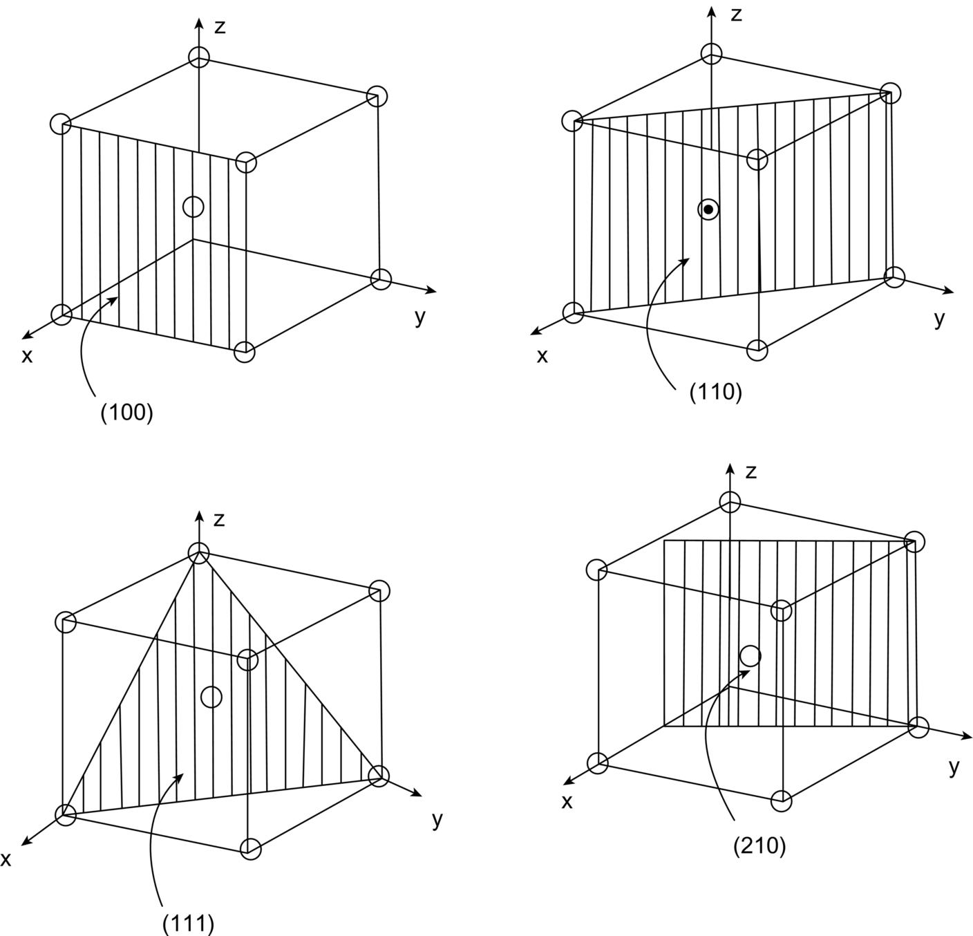
5.5 Plane Indices
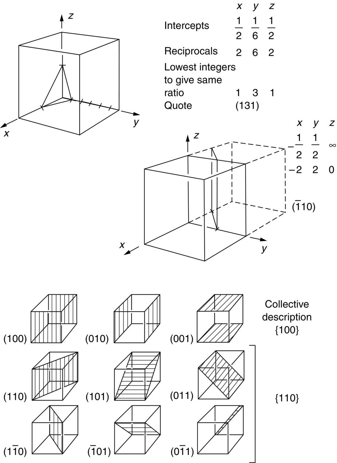
 1 0) planes are defined. The lower part of the figure shows the family of {1 0 0} and of {1 1 0} planes.
 0), (101), (
 01), (011), and (0
 1), or, collectively, {110}. (Here the sign
  means an intercept of –1.) As a final example, our original close-packed planes—the ones of the ABC stacking—are of {111} type. Obviously the unique structural description of “{111} f.c.c.” is a good deal more succinct than a scale drawing of close-packed billiard balls.
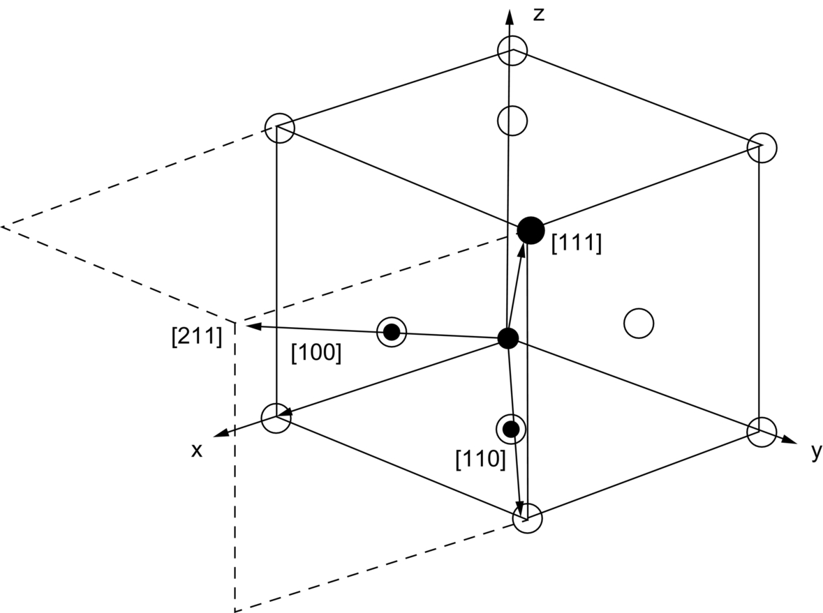
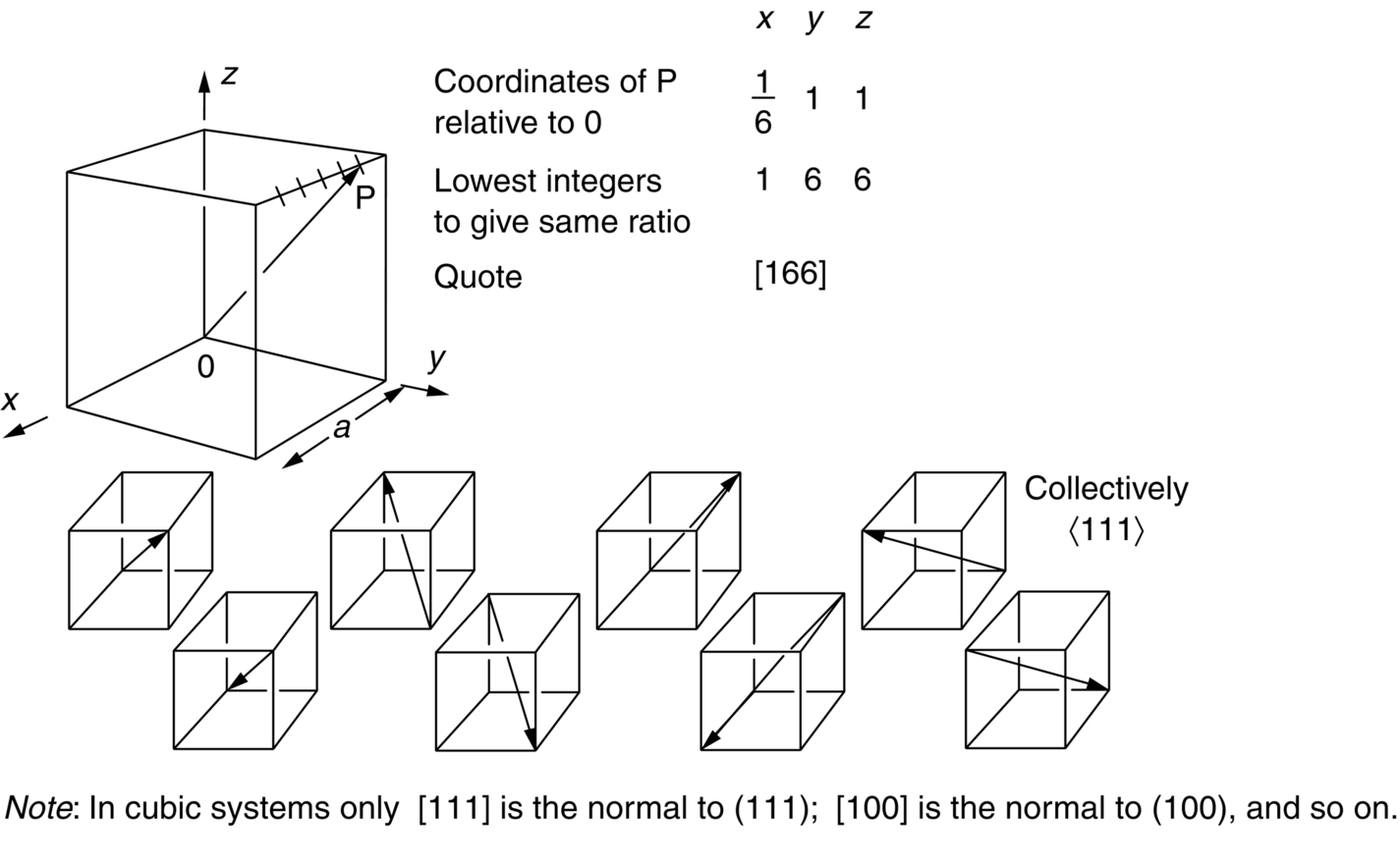
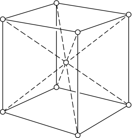
5.6 Direction Indices
Worked Example 1
5.7 Other Crystal Structures
Worked Example 2
5.8 Atom Packing in Polymers
5.9 Atom Packing in Inorganic Glasses
5.10 Density of Solids
Material
ρ (Mg m–3)
Osmium
22.7
Platinum
21.4
Tungsten and alloys
13.4–19.6
Gold
19.3
Uranium
18.9
Tungsten carbide, WC
14.0–17.0
Tantalum and alloys
16.6–16.9
Molybdenum and alloys
10.0–13.7
Cobalt/tungsten–carbide cermets
11.0–12.5
Lead and alloys
10.7–11.3
Silver
10.5
Niobium and alloys
7.9–10.5
Nickel
8.9
Nickel alloys
7.8–9.2
Cobalt and alloys
8.1–9.1
Copper
8.9
Copper alloys
7.5–9.0
Brasses and bronzes
7.2–8.9
Iron
7.9
Iron-based super-alloys
7.9–8.3
Stainless steels, austenitic
7.5–8.1
Tin and alloys
7.3–8.0
Low-alloy steels
7.8–7.85
Mild steel
7.8–7.85
Stainless steel, ferritic
7.5–7.7
Cast iron
6.9–7.8
Titanium carbide, TiC
7.2
Zinc and alloys
5.2–7.2
Chromium
7.2
Zirconium carbide, ZrC
6.6
Zirconium and alloys
6.6
Titanium
4.5
Titanium alloys
4.3–5.1
Alumina, Al2O3
3.9
Alkali halides
3.1–3.6
Magnesia, MgO
3.5
Silicon carbide, SiC
2.5–3.2
Silicon nitride, Si3N4
3.2
Mullite
3.2
Beryllia, BeO
3.0
Common rocks
2.2–3.0
Calcite (marble, limestone)
2.7
Aluminum
2.7
Aluminum alloys
2.6–2.9
Silica glass, SiO2 (quartz)
2.6
Soda glass
2.5
Concrete/cement
2.4–2.5
GFRPs
1.4–2.2
Carbon fibers
2.2
PTFE
2.3
Boron fiber/epoxy
2.0
Beryllium and alloys
1.85–1.9
Magnesium and alloys
1.74–1.88
Fiberglass (GFRP/polyester)
1.55–1.95
Graphite, high strength
1.8
PVC
1.3–1.6
CFRPs
1.5–1.6
Polyesters
1.1–1.5
Polyimides
1.4
Epoxies
1.1–1.4
Polyurethane
1.1–1.3
Polycarbonate
1.2–1.3
PMMA
1.2
Nylon
1.1–1.2
Polystyrene
1.0–1.1
Polyethylene, high-density
0.94–0.97
Ice, H2O
0.92
Natural rubber
0.83–0.91
Polyethylene, low-density
0.91
Polypropylene
0.88–0.91
Common woods
0.4–0.8
Cork
0.1–0.2
Foamed plastics
0.01–0.6
Examples
Answers
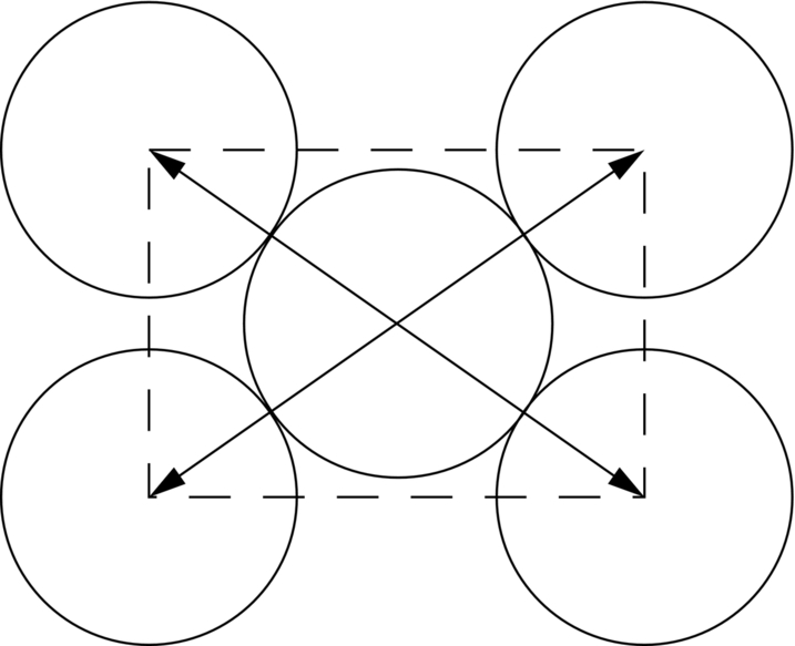
Answer = 4 × (4πr3/3)/a3 = 0.740.
In Chapter 10, we look at how crystals can deform permanently in shear by slipping on crystal planes. See Figures 10.3 and 10.4, which show the slip plane and slip direction in a simple cubic crystal structure.