6.1 Introduction

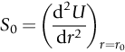
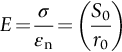
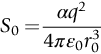
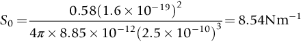
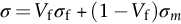
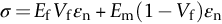
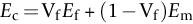
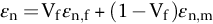
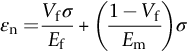
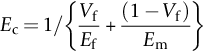
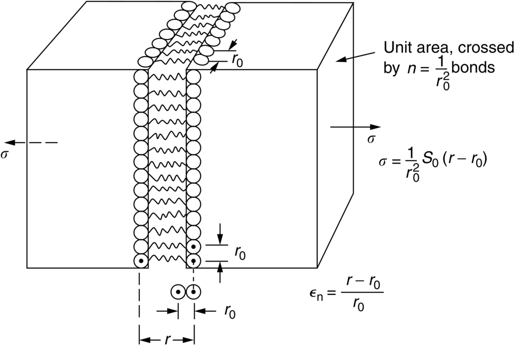
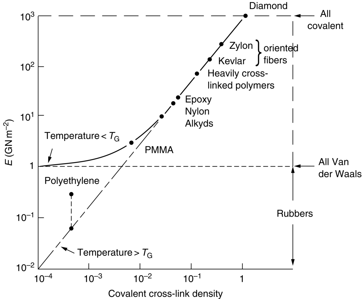
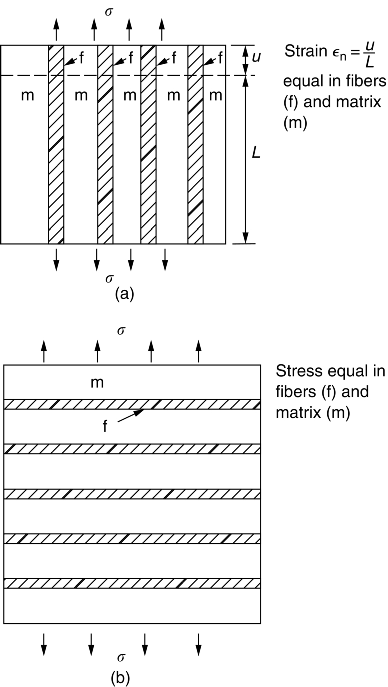
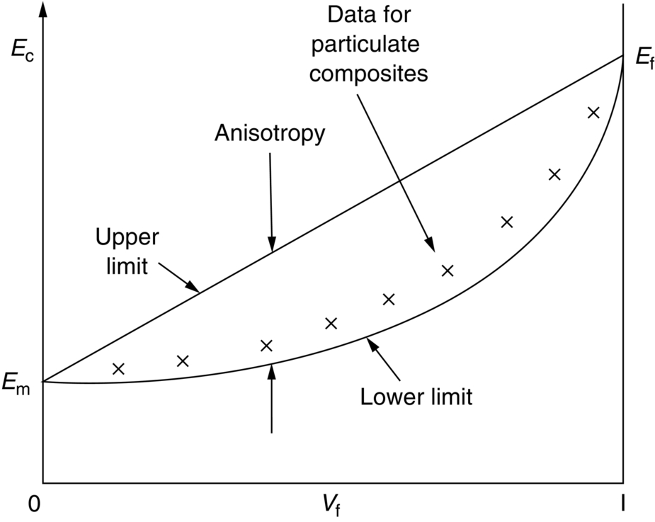
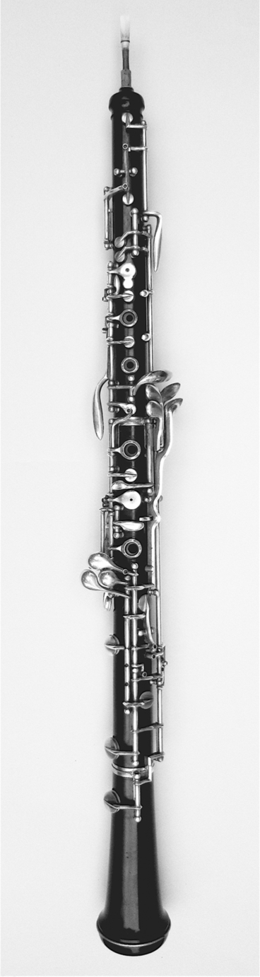
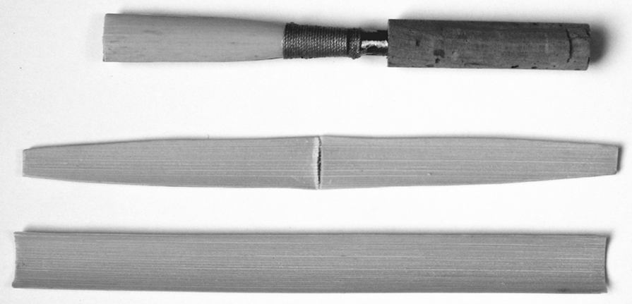
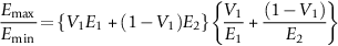
We can now bring together the factors underlying the moduli of materials. First, look back to Figure 3.6, the bar chart showing the moduli of materials. Recall that most ceramics and metals have moduli in a relatively narrow range: 30–300 GN m^–2. Cement and concrete (45 GN m^–2) are near the bottom of that range. Aluminum (69 GN m^–2) is higher up; and steels (200 GN m^–2) are near the top. Special materials lie outside it—diamond and tungsten lie above; ice and lead lie a little below—but most crystalline materials lie in that fairly narrow range. Polymers are different: most of them have moduli that are smaller, some by several orders of magnitude. Why is this? What determines the general level of the moduli of solids? And is there the possibility of producing stiff polymers?

6.2 Moduli of Crystals

We showed in Chapter 4 that atoms in crystals are held together by bonds that behave like little springs. We defined the stiffness of these bonds as

S0=d2Udr2r=r0

Imagine a solid held together by these little springs, linking the atoms between two planes within the material, as shown in Figure 6.1. For simplicity we put atoms at the corners of cubes of side r₀.

The total force exerted across unit area, if the two planes are pulled apart a distance (r – r₀) is the stress σ with

σ=nS0(r–r0)

S₀ can be calculated from the theoretically derived U(r) curves described in Chapter 4. This is the realm of the solid-state physicist and quantum chemist, but we shall consider one example: the ionic bond, for which U(r) is given in Equation (4.3). We showed in Example 4.8 that

S0=αq24πɛ0r03

for the ionic bond. The coulombic attraction is a long-range interaction (it varies as 1/r; an example of a short-range interaction is one that varies as 1/r¹⁰). Because of this, a given Na⁺ ion not only interacts (attractively) with its shell of six neighboring Cl^– ions, it also interacts (repulsively) with the 12 slightly more distant Na⁺ ions, with the eight Cl^– ions beyond that, and with the six Na⁺ ions that form the shell beyond that. To calculate S₀ properly, we must sum over all these bonds, taking attractions and repulsions properly into account. The result is identical with Equation (6.6), but with α = 0.58.

The Table of Physical Constants on the inside front cover gives values for q and ɛ₀. r₀, the atom spacing, is close to 2.5 × 10^–10 m. Inserting these values gives:

S0=0.58(1.6×10–19)24π×8.85×10–12(2.5×10–10)3=8.54Nm–1

The stiffnesses of other bond types are calculated in a similar way (in general, the cumbersome sum just described is not needed because the interactions are of short range). The resulting hierarchy of bond stiffnesses is as shown in Table 6.1.

A comparison of these predicted values of E with the measured values plotted in the bar chart of Figure 3.6 shows that, for metals and ceramics, the values of E we calculate are about right: the bond-stretching idea explains the stiffness of these solids. We can be happy that we can explain the moduli of these classes of solid. But a paradox remains: there exists a whole range of polymers and rubbers that have moduli that are lower—by up to a factor of 100—than the lowest we have calculated. Why is this? What determines the moduli of these floppy polymers if it is not the springs between the atoms?

6.3 Rubbers and Glass Transition Temperature

This is because rubber, like many polymers, is composed of long spaghetti-like chains of carbon atoms, all tangled together, as we showed in Chapter 5. In the case of rubber, the chains are also lightly cross-linked, as shown in Figure 5.10. There are covalent bonds along the carbon chain, and where there are occasional cross-links. These are very stiff, but they contribute very little to the overall modulus because when you load the structure it is the flabby Van der Waals bonds between the chains that stretch, and it is these that determine the modulus.

Well, that is the case at the low temperature, when the rubber has a “proper” modulus of a few GPa. As the rubber warms up to room temperature, the Van der Waals bonds melt. (In fact, the stiffness of the bond is proportional to its melting point: that is why diamond, which has the highest melting point of any material, also has the highest modulus.) The rubber remains solid because of the cross-links, which form a sort of skeleton: but when you load it, the chains now slide over each other in places where there are no cross-linking bonds. This, of course, gives extra strain, and the modulus goes down (remember, E = σ/ɛ_n).

Many of the most floppy polymers have half-melted in this way at room temperature. The temperature at which this happens is called the glass temperature, T_G. Some polymers, which have no cross-links, melt completely at temperatures above T_G, becoming viscous liquids. Others, containing cross-links, become leathery (e.g., PVC) or rubbery (as polystyrene butadiene does). Some typical values for T_G are: polymethylmethacrylate (PMMA, or perspex), 100°C; polystyrene (PS), 90°C; polyethylene (low-density form), –20°C; natural rubber, –40°C.

To summarize, above T_G, the polymer is leathery, rubbery or molten; below, it is a true solid with a modulus of at least 2 GN m^–2. This behavior is shown in Figure 6.2 which also shows how the stiffness of polymers increases as the covalent cross-link density increases, towards the value for diamond (which is simply a polymer with 100 percent of its bonds cross-linked, Figure 4.7). Stiff polymers, then, are possible; the stiffest now available have moduli comparable with that of aluminum. Oriented polymer fibers can be even stiffer.

6.4 Composites

The bar chart of moduli (Figure 3.6) shows that composites can have moduli much higher than those of their matrices. And it also shows that they can be very anisotropic, meaning that the modulus is higher in some directions than others. Wood is an example: its modulus, measured parallel to the fibers, is about 10 GN m^–2; at right angles to this, it is less than 1 GN m^–2.

There is a simple way to estimate the modulus of a fiber-reinforced composite. Suppose we stress a composite, containing a volume fraction V_f of fibers, parallel to the fibers (see Figure 6.3(a)). Loaded in this direction, the strain, ɛ_n, in the fibers and the matrix is the same. The stress carried by the composite is

σ=Vfσf+(1–Vf)σm

where the subscripts f and m refer to fiber and matrix, respectively.

Since σ = Eɛ_n, we can rewrite this as:

σ=EfVfɛn+Em(1–Vf)ɛn

How is it that the modulus can be less? Suppose we had loaded the composite in the opposite way, at right angles to the fibers (as in Figure 6.3(b)). It is now reasonable to assume that the stresses, not the strains, in the two components are equal. If this is so, then the total nominal strain ɛ_n is the weighted sum of the individual strains:

ɛn=Vfɛn,f+(1–Vf)ɛn,m

The two estimates, if plotted, look as shown in Figure 6.4. This explains why fiber-reinforced composites like wood and GFRP are so stiff along the reinforced direction (the upper line of the figure) and yet so floppy at right angles to the direction of reinforcement (the lower line), that is, it explains their anisotropy. Anisotropy is sometimes what you want—as in the shaft of a squash racquet or a vaulting pole. Sometimes it is not, and then the layers of fibers can be laminated in a criss-cross way, as they are in the skins of aircraft flaps.

Not all composites contain fibers. Materials can also be stiffened by small particles. The theory is, as one might imagine, more difficult than for fiber-reinforced composites. But it is useful to know that the moduli of these so-called particulate composites lie between the upper and lower limits of Equations (6.7) and (6.8), nearer the lower one than the upper one, as shown in Figure 6.4. It is much less expensive to mix silica into a polymer than to carefully align specially produced glass fibers in the same polymer. Thus, the modest increase in stiffness given by particles is economically worthwhile.

The resulting particulate composite is isotropic, rather than anisotropic (as would be the case for the fiber-reinforced composites) and this, too, can be an advantage. These filled polymers can be formed and molded by normal methods (most fiber composites cannot) and so are cheap to fabricate. Many of the polymers of everyday life—bits of cars and bikes, household appliances and so on—are filled in this way.

Worked Example

The photograph on the next page shows an oboe—one of the woodwind instruments of the classical symphony orchestra; see http://en.wikipedia.org/wiki/Oboe.

The close-up shows the most critical component of the instrument—the reed. The player places the reed in his/her mouth, and blows through it in order to drive the natural frequencies of air inside the main tube of the instrument. The “reed” is actually made from a species of cane—Arundo Donax. This grows in marshy coastal areas in the south of France, as well as other places (California and Argentina, for example) where there is the right soil and climate—essential to growing the best cane.

A piece of the tubular cane is first split along its length, and the inside is “gouged” to produce the right thickness. The gouged piece is then cut to the correct length and width, folded in half, and tied on to a small brass tube (the “staple”). After tying-on, the folded end is cut off, and the reed is “scraped” to the correct thickness profile using a reed-scraping knife. The final scraping is critical to the correct functioning of the reed. In fact, most professional oboeists spend much more time making and adjusting reeds than they ever do playing the instrument!

The two separated halves of the reed behave like cantilever springs, and when the oboeist blows through the reed, the cantilevers beat rapidly against one another. This is what powers the vibrations inside the instrument. But this is just the start—with as little stress as possible, the player must be able to play loudly and softly, start notes quietly over the whole range of the instrument, play staccato and legato, make a nice sound, and so on. A well-made and adjusted cane reed does all these things well, because it has just the right combination of properties—stiffness, density, damping, water uptake (conditioning). But a critical factor is that Young’s modulus for cane is anisotropic—Young’s modulus along the tube axis is approximately 10 times that transverse to the axis. The performance of any synthetic substitutes will be wholly inadequate unless they can match the anisotropy of natural cane.

Examples

Answers