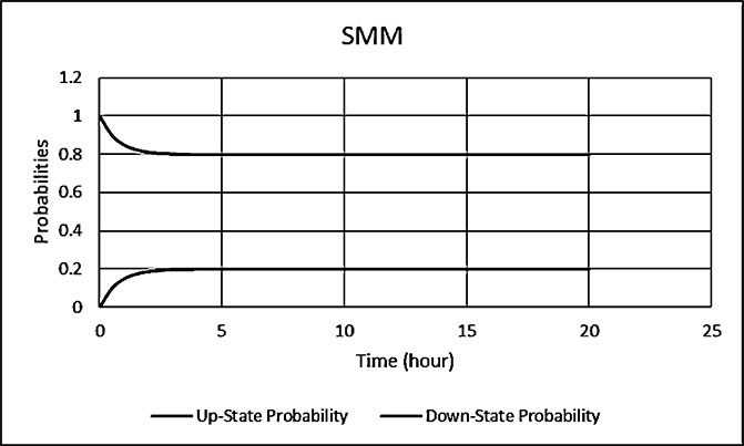
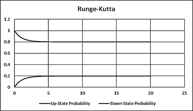
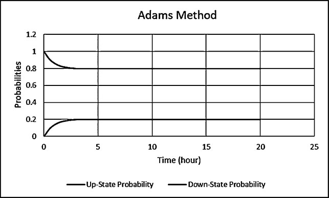
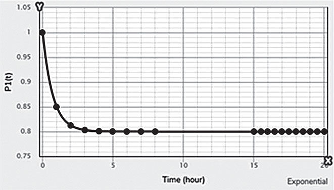
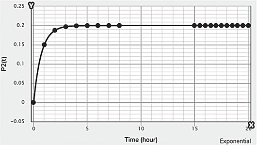
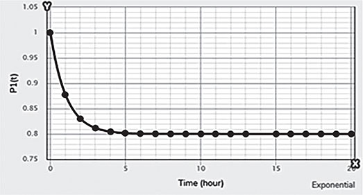
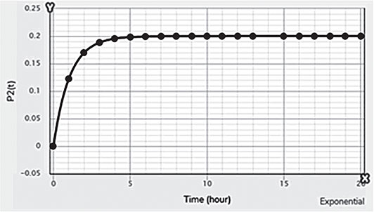
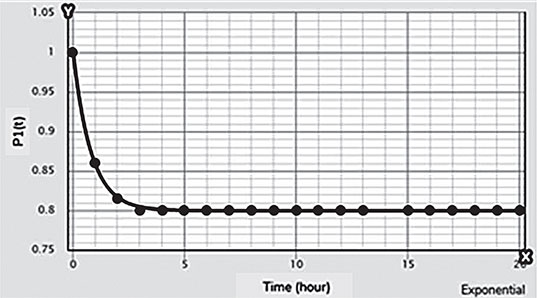
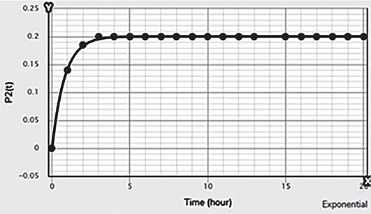
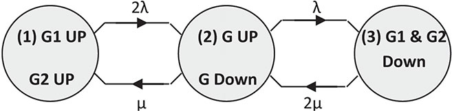
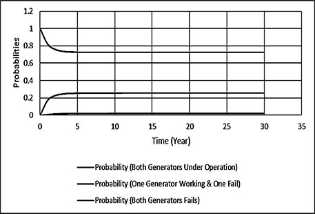
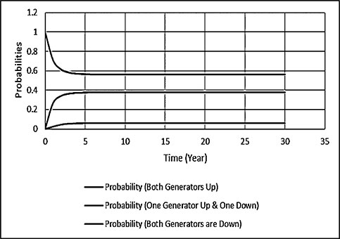
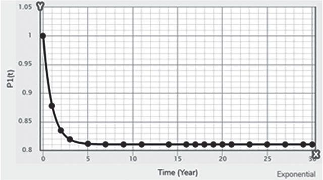
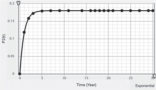
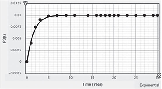
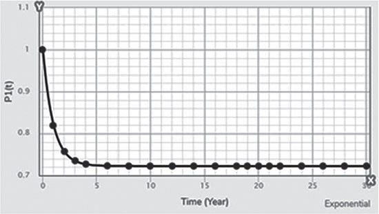
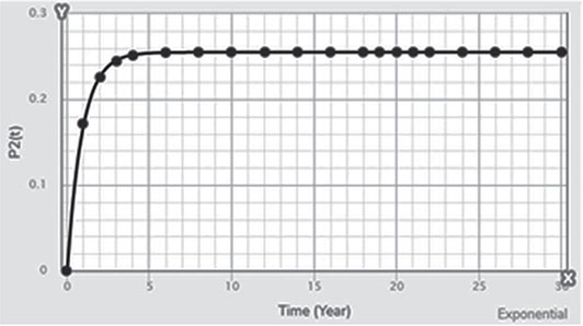
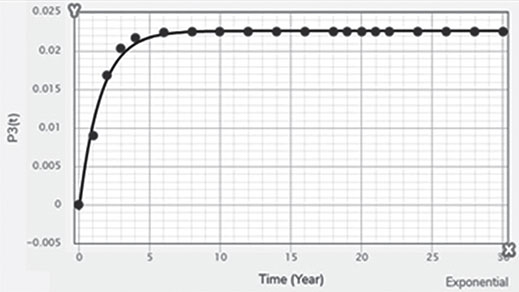
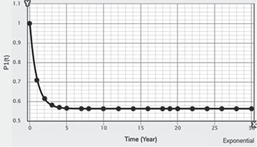
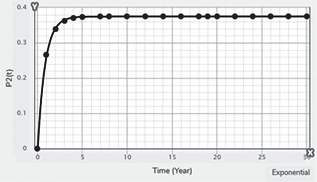
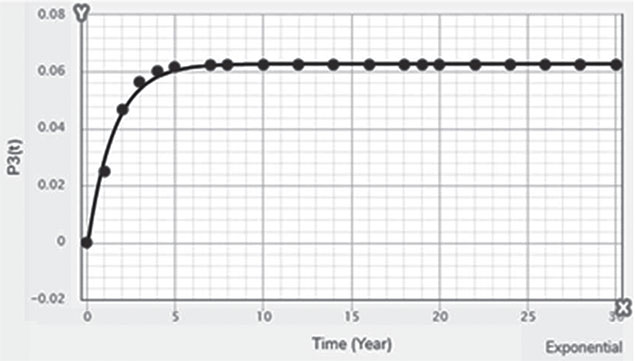
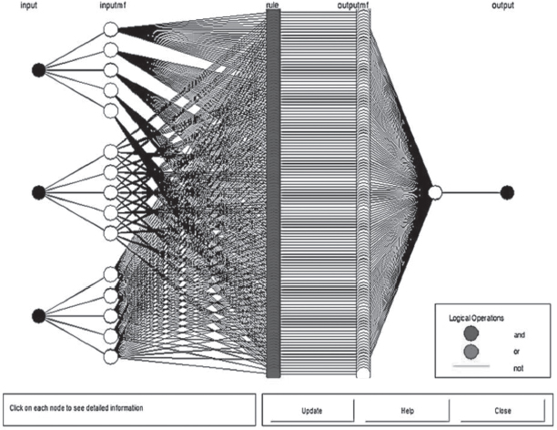
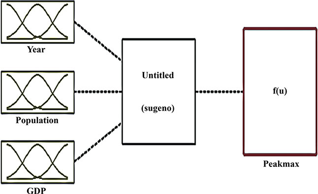
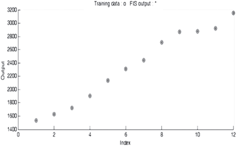
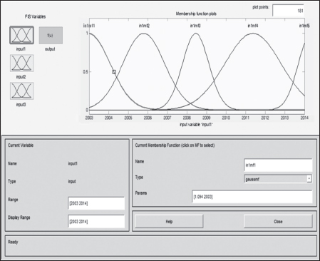
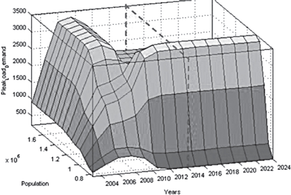
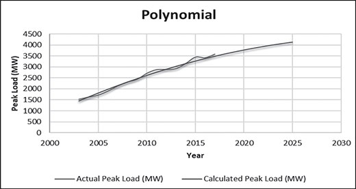
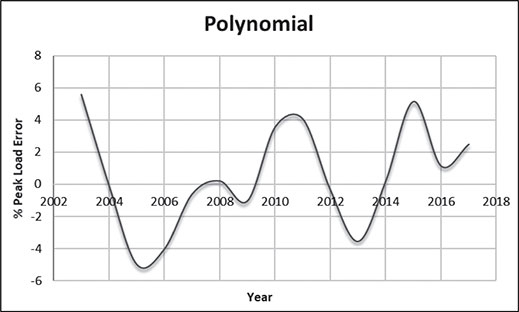
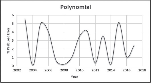
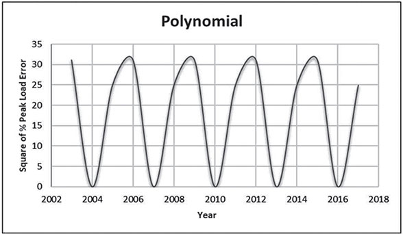
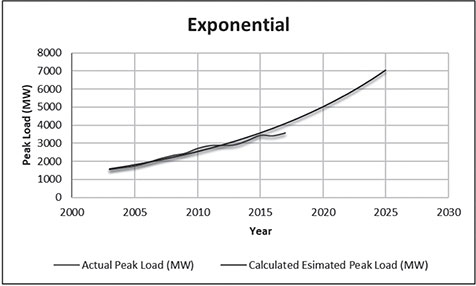
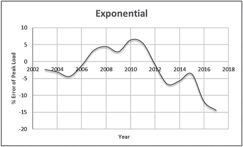
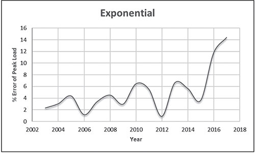
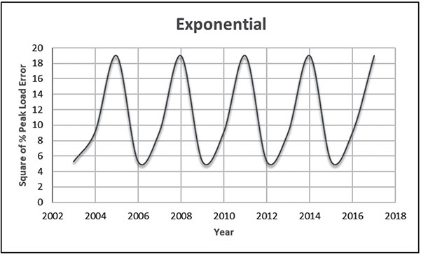
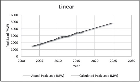
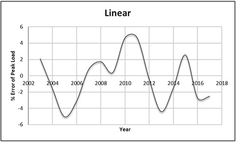
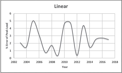
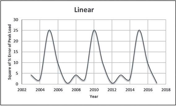
Electrical energy is an essential ingredient for the development of modern society. Almost all aspects of daily life depend on the use of electrical energy and the performance of a power utility. The power utility is measured in terms of the quality and reliability of the supply. Electric power utilities have invested a substantial amount of capital in generating stations, transmission lines, and distribution facilities to supply electrical energy to their customers as economically as possible and with a reasonable assurance of continuity, safety, and quality. This creates the difficult problem of balancing the need for continuity of power supply with the costs involved. There are a number of methods for constructing the transition rate matrix. For general systems using the Kronecker algebra helps to form a transition rate matrix. This is one method out of a number of methods that help to form a transition rate matrix. Also, the rules and properties can be introduced. The Kronecker algebra is used in this textbook for constructing the transition rate matrix of a system contain a number of power stations. The two-state model refers to a generator passing through two-states. In this case, the power generator is passing through Up-State and Down-State. This means the generator is operating and is failing, respectively. The three methods to calculate the transient probabilities for the considered system are discussed earlier in Chapter 8. The results are obtained using the SMM illustrated in Table 10.1 and Figure 10.1. Table 10.2 and Figure 10.2 illustrate the results obtained by the Rung-Kutta method. Finally, Table 10.3 and Figure 10.3 show the results obtained by the Adams method. These three methods are recommended to calculate the transient and steady-state probabilities for any model. Time (year) P1(t) P2(t) 0 1 0 0.5 0.9 0.1 1 0.85 0.15 1.5 0.825 0.175 2 0.8125 0.1875 2.5 0.8063 0.1938 3 0.8031 0.1969 3.5 0.8016 0.1984 4 0.8008 0.1992 4.5 0.8004 0.1996 5 0.8002 0.1998 5.5 0.8001 0.1999 6 0.8 0.2 6.5 0.8 0.2 7 0.8 0.2 7.5 0.8 0.2 8 0.8 0.2 15 0.8 0.2 15.5 0.8 0.2 16 0.8 0.2 16.5 0.8 0.2 17 0.8 0.2 17.5 0.8 0.2 18 0.8 0.2 18.5 0.8 0.2 19 0.8 0.2 19.5 0.8 0.2 20 0.8 0.2 Time (year) P1(t) P2(t) 0 1 0 0.5 0.9245 0.0755 1 0.8775 0.1225 1.5 0.8482 0.1518 2 0.83 0.17 2.5 0.8187 0.1813 3 0.8116 0.1884 3.5 0.8072 0.1928 4 0.8045 0.1955 4.5 0.8028 0.1972 5 0.8017 0.1983 5.5 0.8011 0.1989 6 0.8007 0.1993 6.5 0.8004 0.1996 7 0.8003 0.1997 7.5 0.8002 0.1998 8 0.8001 0.1999 8.5 0.8001 0.1999 9 0.8 0.2 9.5 0.8 0.2 10 0.8 0.2 10.5 0.8 0.2 11 0.8 0.2 11.5 0.8 0.2 12 0.8 0.2 12.5 0.8 0.2 13 0.8 0.2 13.5 0.8 0.2 14 0.8 0.2 14.5 0.8 0.2 15 0.8 0.2 15.5 0.8 0.2 16 0.8 0.2 16.5 0.8 0.2 17 0.8 0.2 17.5 0.8 0.2 18 0.8 0.2 18.5 0.8 0.2 19 0.8 0.2 19.5 0.8 0.2 20 0.8 0.2 Time (hr) P1(t) P2(t) 0 1 0 0.5 0.91 0.09 1 0.86 0.14 1.5 0.83 0.17 2 0.815 0.185 2.5 0.805 0.195 3 0.8 0.2 3.5 0.8 0.2 4 0.8 0.2 4.5 0.8 0.2 5 0.8 0.2 5.5 0.8 0.2 6 0.8 0.2 6.5 0.8 0.2 7 0.8 0.2 7.5 0.8 0.2 8 0.8 0.2 8.5 0.8 0.2 9 0.8 0.2 9.5 0.8 0.2 10 0.8 0.2 11 0.8 0.2 11.5 0.8 0.2 12 0.8 0.2 13 0.8 0.2 14 0.8 0.2 15 0.8 0.2 16 0.8 0.2 17 0.8 0.2 18 0.8 0.2 19 0.8 0.2 20 0.8 0.2 The curve fitting technique, applied to the three methods, is used to find out the results for the two-state model. The results are illustrated in Figures 10.4a, b using SMM, Figures 10.5a, b using the Runge-Kutta method, and Figures 10.6a, b using Adams method. The suitable equations for the three methods are summarized in Table 10.4. The three-state model (Figure 10.7) is considered for a case of two generators under operation in a power station. The first state considered that both generators are working, where the second state illustrates that one is working and the others fail. In the third state, both generators are in a failstate. Using the Laplace transforms will result: Method Probability a b c SMM 1 0.7999963±0.000003416 0.2000039±0.00001428 1.386269±0.0002655 2 0.2000037±0.000003416 –0.2000039±0.00001428 1.386269±0.0002655 Runge-Kutta 1 0.7999955±0.000005142 0.2000096±0.00002047 0.948314±0.000219 2 0.2000045±0.000005142 –0.2000096±0.00002047 0.948314±0.000219 Adams 1 0.7996066±0.0003309 0.2007632±0.001368 1.236986±0.02122 2 0.2003934±0.0003309 –0.2007631±0.001368 1.236985±0.02122 The results are illustrated in three cases. These cases are summarized in Tables 10.5, 10.6, 10.7, 10.8 and Figures 10.8, 10.9, 10.10. Case # μ (per year) λ (per year) Table Figure 1 0.9 0.1 2 0.85 0.15 3 0.75 0.25 TIME (YEAR) P1(T) P2(T) P3(T) 0 1 0 0 1 0.877571652 0.118432584 0.003995764 2 0.834543507 0.157980042 0.007476451 3 0.81898646 0.171984494 0.009029046 4 0.81330017 0.177062789 0.009637042 5 0.811213284 0.17892102 0.009865695 6 0.810446237 0.179603277 0.009950486 7 0.810164147 0.179854082 0.009981771 8 0.810060384 0.179946324 0.009993292 9 0.810022214 0.179980254 0.009997532 10 0.810008172 0.179992736 0.009999092 11 0.810003006 0.179997328 0.009999666 12 0.810001106 0.179999017 0.009999877 13 0.810000407 0.179999638 0.009999955 14 0.81000015 0.179999867 0.009999983 15 0.810000055 0.179999951 0.009999994 16 0.81000002 0.179999982 0.009999998 17 0.810000007 0.179999993 0.009999999 18 0.810000003 0.179999998 0.01 19 0.810000001 0.179999999 0.01 20 0.81 0.18 0.01 21 0.81 0.18 0.01 22 0.81 0.18 0.01 23 0.81 0.18 0.01 24 0.81 0.18 0.01 25 0.81 0.18 0.01 26 0.81 0.18 0.01 27 0.81 0.18 0.01 28 0.81 0.18 0.01 29 0.81 0.18 0.01 30 0.81 0.18 0.01 Time (year) P1(t) P2(t) P3(t) 0 1 0 0 1 0.819354301 0.17165523 0.008990469 2 0.757422599 0.225755387 0.016822014 3 0.735251474 0.244433172 0.020315354 4 0.727178036 0.25113862 0.021683344 5 0.724219198 0.253582988 0.022197814 6 0.72313222 0.254479186 0.022388594 7 0.722732549 0.254808467 0.022458984 8 0.722585546 0.254929548 0.022484907 9 0.72253147 0.254974083 0.022494447 10 0.722511577 0.254990466 0.022497957 11 0.722504259 0.254996493 0.022499248 12 0.722501567 0.25499871 0.022499724 13 0.722500576 0.254999525 0.022499898 14 0.722500212 0.254999825 0.022499963 15 0.722500078 0.254999936 0.022499986 16 0.722500029 0.254999976 0.022499995 17 0.722500011 0.254999991 0.022499998 18 0.722500004 0.254999997 0.022499999 19 0.722500001 0.254999999 0.0225 20 0.722500001 0.255 0.0225 21 0.7225 0.255 0.0225 22 0.7225 0.255 0.0225 23 0.7225 0.255 0.0225 24 0.7225 0.255 0.0225 25 0.7225 0.255 0.0225 26 0.7225 0.255 0.0225 27 0.7225 0.255 0.0225 28 0.7225 0.255 0.0225 29 0.7225 0.255 0.0225 30 0.7225 0.255 0.0225 Time (year) P1(t) P2(t) P3(t) 0 1 0 0 1 0.708913246 0.266113229 0.024973525 2 0.614395459 0.338876724 0.046727817 3 0.581325073 0.362243389 0.056431538 4 0.569389331 0.370379157 0.060231512 5 0.565029568 0.373309838 0.061660594 6 0.563429916 0.374379544 0.06219054 7 0.562842008 0.374771926 0.062386067 8 0.562625806 0.37491612 0.062458074 9 0.56254628 0.374969146 0.062484575 10 0.562517025 0.37498865 0.062494325 11 0.562506263 0.374995825 0.062497912 12 0.562502304 0.374998464 0.062499232 13 0.562500848 0.374999435 0.062499717 14 0.562500312 0.374999792 0.062499896 15 0.562500115 0.374999924 0.062499962 16 0.562500042 0.374999972 0.062499986 17 0.562500016 0.37499999 0.062499995 18 0.562500006 0.374999996 0.062499998 19 0.562500002 0.374999999 0.062499999 20 0.562500001 0.374999999 0.0625 21 0.5625 0.375 0.0625 22 0.5625 0.375 0.0625 23 0.5625 0.375 0.0625 24 0.5625 0.375 0.0625 25 0.5625 0.375 0.0625 26 0.5625 0.375 0.0625 27 0.5625 0.375 0.0625 28 0.5625 0.375 0.0625 29 0.5625 0.375 0.0625 30 0.5625 0.375 0.0625 The Laplace Transforms and Adams Methods have been applied to obtain the transient probabilities shown in the present chapter. The curve fitting technique applied to the three cases of the three-state model. The results obtained are summarized in Figures 10.11a,b,c, 10.12a,b,c, and 10.13a,b,c as the values of the repair and failure rates printed. The results of the fitting equations for the three cases are summarized in Table 10.9. Any number of Markov models (representing a number of systems) can form one large system representing an electric power station. This clear when the Kronecker multiplication is used. Method Probability a b c LT, 1 0.8100282±0.00003175 0.1899086±0.0001303 1.029159±0.001632 μ = 0.9 2 0.1799455±0.00005997 –0.1798336±0.0002469 1.063473±0.003417 λ = 0.1 3 0.01003722±0.00005733 –0.01026308±0.00005997 0.6513805±0.02942 LT, 1 0.7225763±0.00007297 0.277281±0.0002973 1.045382±0.002606 μ = 0.85 2 0.254857±0.0001317 –0.2546274±0.00054 1.104067±0.00557 λ = 0.15 3 0.0225983±0.0001371 –0.02314623±0.0005211 0.6590729±0.03037 LT, 1 0.5627287±0.0001916 0.4369243±0.0007806 1.082793±0.004574 μ = 0.75 2 0.3746189±0.0003001 –0.3742009±0.001239 1.215129±0.01003 λ = 0.25 3 0.06282769±0.0003926 –0.06439482±0.001466 0.6609917±0.03079 The Kronecker product is very efficient to form a large model of the electric power system, where this an advantage recorded for the Kronecker product. Figure 10.14 illustrates the four layers connection for three inputs and one output. These four layers represent the Neuro-Fuzzy model, which is used to represent the developed estimated peak load model in this study. It is clear that the results obtained automatically through the training of data performed in the Adaptive Neuro-Fuzzy Inference System (ANFIS). Figure 10.15 shows the proposed model using the Neuro-Fuzzy, where the proposed model is three inputs and one output model. The three inputs are the year, population, and GDP. The output is the peak load for the country. Therefore, the three inputs used as follows: 1. Input 1: Year. 2. Input 2: Population. 3. Input 3: GDP. Figure 10.16 illustrates the actual data collected and presented for member state’s peak demand, where the estimated peak load demand for the coming years generated by Neuro-Fuzzy model. Figure 10.17 membership function used in the neuro-fuzzy logic model for long term load forecasting. The ANFIS or adaptive network-based fuzzy inference system can be a shortage as “ANFIS.” ANFIS is a kind of artificial neural networkmodeling standard. It was adopted to effectively tune the membership function to decrease the output error and maximize performance indicators. At the same time, ANFIS Editor Display made up four types. These types are Load data, General is, Train FIS, and Test FIS. The load data is used for training, testing, and checking. In the research, the ANFIS approach is recommended, where it is used by adding the Artificial Neural Network to the Fuzzy System, which has successfully simulated for the load forecasting. The electricity load forecasting is an active research topic with important practical effects for almost any industry. It is well known that the load forecasting is a technique used by electric power or electric energyproviding companies to estimate the power or energy needed to satisfy the demand and supply stability. The accuracy of forecasting is of great worth for the operational and managerial loading of a utility company. The most accurate estimation of energy consumption and supplies has a helpful impact on active budgets. In the instance of the electrical industry, accurate electrical load estimating is a suitable means to provide well-grounded information and capable energy management for arrangement in both the mid and long term and for the network operation in the short term. Back to the term (surface). The term (surface) is viewer represented by a graphical interface that lets the researcher examines the output surface of the fuzzy inference system (FIS) for two inputs. Figure 10.18 illustrates an example of a load forecasting of a country. The inputs are the population and years to find the estimates load for further years, as shown in Figure 10.18. To design high-precision estimators for a load-cell-based weighting system with temperature compensation, ANFIS is used to model the relationship with actual weights of samples. In addition, ANFIS can improve the precision of load cell. ANFIS is used to model the relationship between the reading of load cells and the actual weight of samples considering the temperature-varying effect and nonlinearity of the load cells. The model of the load-cell-based weighting system can accurately estimate the weight of test samples from the load cell reading. The proposed ANFIS-based method is convenient to use and can improve the 117 precision of digital load cell measurement systems. The temperature and humidity are two parameters considered. The humidity and the temperature data are fed to the fuzzy logic (FL) system, where the output is the load. The load is proportional to these two parameters. The neural networks used for training and comparing the set of the past load to predict the future. In this case, the load does not just depend on the temperature and humidity but also depends on the other data like a number of customers for Load Forecasting of the Power System Planning using Fuzzy-Neural. There are a number of methods used to estimate the electric load for the countries. Kingdom of Bahrain taken as an example in the present chapter to estimate its electric load for the future up to the year 2025 using the polynomial. Table 10.10 shows the estimated peak loads for the Kingdom of Bahrain with calculated results using the Polynomial. The electric load percentage error using the polynomial is calculated and found as 2.471288523. The estimated load versus the years is plotted and illustrated in Figure 10.19. The percentage error of the peak load for the results of the polynomial is shown in Figure 10.20. The results of the percentage error for the peak load converted to absolute values and shown in Figure 10.21. Furthermore, when the square of the peak load error versus the years obtained, which is shown in Figure 10.22, the shape of that becoming almost a sinusoidal. There are a number of methods used to estimate the electric load for the countries. Kingdom of Bahrain taken as an example in the present chapter to estimate its electric load for the future up to the year 2025 using the exponential. Table 10.11 shows the peak loads for the Kingdom of Bahrain with calculated estimated peak loads results using the Exponential. The electric load percentage error using the exponential is calculated and found as5.100549189. The estimated load versus the years is plotted and illustrated in Figure 10.23. The percentage error of the peak load for the results of the exponential is shown in Figure 10.24. The results of the absolute value percentage error for the peak load is found and shown in Figure 10.25. Furthermore, when the square of the peak load error versus the years obtained, which is shown in Figure 10.26, the shape of that becoming almost a sinusoidal. Year Peak Load Actual (MW) Peak Load Calculated (MW) % Peak Load Error 2003 1535 1449.329226 5.581157948 2004 1632 1633.227512 –0.075215196 2005 1725 1811.186738 –4.996332609 2006 1906 1983.206902 –4.050729381 2007 2136 2149.288006 –0.622097636 2008 2314 2309.430048 0.197491443 2009 2438 2463.63303 –1.051395796 2010 2708 2611.89695 3.54885709 2011 2871 2754.22181 4.067509248 2012 2880 2890.607608 –0.368319722 2013 2917 3021.054346 –3.567169883 2014 3152 3145.562022 0.204250571 2015 3441 3264.130638 5.140057033 2016 3415 3376.760192 1.119760117 2017 3572 3483.450686 2.478984169 2018 3584.202118 2019 3679.01449 2020 3767.8878 2021 3850.82205 2022 3927.817238 2023 3998.873366 2024 4063.990432 2025 4123.168438 Year Actual Peak Load (MW) Estimated Peak Load (MW) % Error 2003 1535 1570.298109 –2.299551106 2004 1632 1681.342525 –3.023439059 2005 1725 1800.239503 –4.361710307 2006 1906 1927.544339 –1.130343093 2007 2136 2063.851601 3.377734032 2008 2314 2209.797899 4.503115861 2009 2438 2366.064862 2.950579889 2010 2708 2533.382322 6.448215581 2011 2871 2712.53172 5.519619656 2012 2880 2904.349756 –0.845477656 2013 2917 3109.732302 –6.60720952 2014 3152 3329.638576 –5.635741633 2015 3441 3565.095633 –3.606382826 2016 3415 3817.203153 –11.77754475 2017 3572 4087.138583 –14.42157287 2018 4376.162631 2019 4685.62516 2020 5016.971486 2021 5371.749133 2022 5751.615059 2023 6158.343393 2024 6593.833726 2025 7060.119975 There are a number of methods used to estimate the electric load for the countries. Kingdom of Bahrain taken as an example in the present chapter to estimate its electric load for the future up to the year 2025 using the linear. Table 10.12 shows the peak loads for the Kingdom of Bahrain with calculated results using the Linear. The electric load percentage error using the linear is calculated and found as 2.533884781. The estimated load versus the years is plotted and illustrated in Figure 10.27. The percentage error of the peak load for the results of the linear is shown in Figure 10.28. The results of the percentage error for the absolute value peak load are found and shown in Figure 10.29. Furthermore, when the square of the peak load error versus the years obtained, which is shown in Figure 10.30, the shape of that becoming almost a semi-sinusoidal. Three techniques were used to find the estimated peak load for the Kingdom of Bahrain using the polynomial, exponential, and linear. The average percentage error was determined and found to be 2.471288523 using the polynomial technique. The average percentage errors were determined and found to be 5.100549189using the Exponential technique. The average percentage errors were determined and found to be 2.533884781using the linear technique. Comparing the three techniques results of the average percentage error, where it is found that the polynomial results have the minimum percentage average error, then the linear results and finally the exponential results. Therefore, the exponential technique is recommended for further research work. When the percentage error of the peak load squared, the sinusoidal form is becoming as a result for both the polynomial and the exponential, where the linear will take the shape of semi-sinusoidal form. In this case, the shape of the sinusoidal, which has been taken, will be homogeneous. Out of the results highlighted, it is recommended to use the polynomial, because it has less percentage error (better accuracy) and a sinusoidal form, which is homogeneous. Year Actual Peak Load (MW) Estimated Peak Load (MW) % Error (Peak Load) 2003 1535 1503.0584 2.080885993 2004 1632 1657.2612 –1.547867647 2005 1725 1811.464 –5.012405797 2006 1906 1965.6668 –3.130472193 2007 2136 2119.8696 0.755168539 2008 2314 2274.0724 1.725479689 2009 2438 2428.2752 0.398884331 2010 2708 2582.478 4.635228951 2011 2871 2736.6808 4.678481365 2012 2880 2890.8836 –0.377902778 2013 2917 3045.0864 –4.391031882 2014 3152 3199.2892 –1.500291878 2015 3441 3353.492 2.543097937 2016 3415 3507.6948 –2.714342606 2017 3572 3661.8976 –2.516730123 2018 3816.1004 2019 3970.3032 2020 4124.506 2021 4278.7088 2022 4432.9116 2023 4587.1144 2024 4741.3172 2025 4895.52 • adaptive network-based fuzzy inference system • adaptive neuro-fuzzy inference system • equivalent transition rate matrix • load forecasted surface • membership function • three-state models Ameen, I., & Novati, P. The solution of fractional order epidemic model by implicit Adams methods. Applied Mathematical Model, 2017, 43, 78–84. Billinton, R., & Allan, R. N. Reliability Evaluation of Engineering Systems: Concepts and Techniques (2nd edn.). Pitman: New York, 1992. Qamber, I. S., & Al-Hamad, M. Y. Trading opportunities forecasted benefits at peak load for GCC countries. Electric Power and Water Desalination Conference, 2016, Doha, Qatar. Yanga, X., & Ralescu, D. Adams method for solving uncertain differential equations. Applied Mathematics and Computation, 2015, 270, 993–1003.
CHAPTER 10
Power Systems Reliability Applications
10.1 INTRODUCTION
10.2 EQUIVALENT TRANSITION RATE MATRIX
10.3 TWO-STATE MODEL
10.4 THREE-STATE MODELS
Source: Modified from Billinton and Allan, 1992.

10.5 SYSTEM COMBINATION
10.6 PROPOSED MODEL ADVANTAGE
10.7 MEMBERSHIP FUNCTION
Source: Reprinted from Qamber and Al-Hamad, 2016.
Source: Reprinted from Qamber and Al-Hamad, 2016.
10.7.1 VALIDATION OF MEMBERSHIP FUNCTIONS
Source: Reprinted from Qamber and Al-Hamad, 2016.
Source: Reprinted from Qamber and Al-Hamad, 2016.
10.7.2 LOAD FORECASTED SURFACE
Source: Reprinted from Qamber and Al-Hamad, 2016.
10.8 THE EFFECT OF TEMPERATURE
10.8.1 FIRST MODEL
10.8.2 SECOND MODEL
10.8.3 THIRD MODEL
10.9 COMPARISON BETWEEN THE MODELS
KEYWORDS
REFERENCES