8 Radar Imaging Techniques

8.1 STOCHASTIC WAVE EQUATIONS

Radar as a coherent imager is physically based on the wave equations that govern the behavior of wave-targets interactions through the process of radiation, transmission, propagation, and reflection/refraction. For a randomly rough surface being imaged, the governing waver equations become stochastic [1], as we already considered in Chapter 5. Here, we briefly introduce the stochastic wave equations at a minimum but sufficient level to serve as fundamentals of radar imaging.

Consider the radar imaging of a nonmagnetic random medium as shown in Figure 8.1. The locations of the transmitter T_x and receiver R_x are in bistatic mode. For more the general random medium, it is specified by the constitute relations as given in 3.2 of Chapter 3.

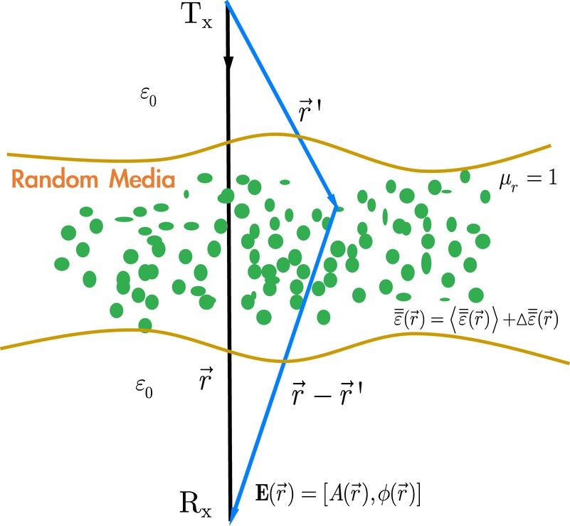
**FIGURE 8.1** Radar imaging of a random medium.

Similarly to the problem we deal with the Huygen’s principle, the total field E received at Rx is the sum of the transmitted field E^t at Tx and scattered field E^s from the random medium under the presence of the incident field, as already introduced in Equation 1.18:

$E (\vec{r}) = E^{i} (\vec{r}) + k_{0}^{2} \int \bar{\bar{G}} (\vec{r}, \vec{r}') \cdot [{\bar{\bar{ε}}}_{r} (\vec{r}') - 1] E (\vec{r}') d \vec{r}' = E^{i} (\vec{r}) + E^{s} (\vec{r})$ (8.1)

where $\bar{\bar{G}}$ is tensor Green’s function; k₀ is the free space wavenumber. ${\bar{\bar{ε}}}_{r} (\vec{r}) - 1 = 0$ is objection function, and may be any other forms. The random medium is described by permittivity $\bar{\bar{ε}} (\vec{r}) = ⟨ \bar{\bar{ε}} (\vec{r}) ⟩ + Δ \bar{\bar{ε}} (\vec{r})$ , where $⟨ \bar{\bar{ε}} (\vec{r}) ⟩$ is the mean permittivity and $Δ \bar{\bar{ε}} (\vec{r})$ is the fluctuating permittivity, with ${\bar{\bar{ε}}}_{r} (\vec{r}) = \bar{\bar{ε}} (\vec{r}) / ε_{0}$ . In the absence of the random medium, the objection function ${\bar{\bar{ε}}}_{r} (\vec{r}) - 1 = 0$ , the total field equals the transmitted field. Noted that depending on the location of the receiver, the transmitted field may propagate through the medium. But it would not affect the problem solving, which is by way of applying the boundary conditions.

The scattered field appearing in Equation 8.1 is given rise by scattered by random scatters, scattering from random rough surface, or fluctuating propagation in random continua inside the random medium intercepted by the transmitting antenna and receiving antenna. Because of the random properties of the permittivity, the total field is composed of a mean-field and a fluctuating field [1–3]. In radar, it is commonly named as a coherent and inherent field, correspondingly, similar to our treatment of scattering field in Chapters 4 and 5. Theoretically, decomposing of the total field into a coherent field and incoherent field is mathematically straightforward. In practice, it is not so as the antenna patterns always exercise influence, making it is difficult to differentiate the coherent returns from incoherent returns in total returns. In transmitting the signal toward the medium, an unmodulated waveform is rarely used. Broadly, there are two basic types of waveform: pulse and continuous wave. As such, in microwave remote sensing, linear frequency modulated (LFM) pulse (chirp), frequency modulated continuous wave (FMCW), and step frequency modulated (SFM), are among commonly used waveforms. Proper choice of waveform determines the radar capability of resolving range and azimuth ambiguities and spatial resolutions, and of course depends on the application scenario. It also involves the radar sensitivity, measurement precision, and dynamic ranges [4].

Equation 8.1 constitutes a stochastic vector wave equation to determine the received field. The problem risen here is how to solve Equation 8.1. This is indeed a computational electromagnetic problem. Many excellent books are available to offer solutions for various kinds of boundary values problems [5–9]. A thorough treatment of such problems is not possible and is beyond the scope of this book. Readers can always consult the source of these books to seek a preferred approach. Indeed, with the advances of both software programing (e.g., massively parallel) and hardware development (e.g., graphic computation unit), the computational electromagnetic problem is still in its accelerating progress toward offering higher computationally efficient and accurate solutions as never before. For random medium imaging, an analytical solution to Equation 8.1 is rarely feasible. Two types of numerical solutions are usually devised: full-wave solution and approximate solution. In a full-wave solution, the problem can be treated in time domain or frequency domain, or hybrid. The method of moment (MoM) in the frequency domain and Finite difference time domain (FDTD) is well-known. The full wave approach implies that the solution contains all bounces of scattering, between radar-targets, and among targets. Imaging formation based on full wave solution therefore poses much lesser information loss in terms of preserving the complete scattering process.

Major advances have been made in numerical solutions of Maxwell equations in three-dimensional simulations (NMM3D) [10,11] for rough surface scattering. As an application example, with the fast and yet accurate numerical simulation method at hand, it is not difficult to study the effects of the surface inhomogeneity. By viewing the Green’s function of layered inhomogeneous media, it is noted that the reflect term that accounts for the inhomogeneous effects is needed in addition to a direct term. Mathematically, this is simple and straightforward. Numerically, it is not really so, however. After some mathematical manipulations, it is possible to split the reflect term and cast them into the original algorithm with minimum modifications. we describe the governing equations and the calculation of incident fields and scattered fields of a dielectric rough surface with a finite extent. In numerical solutions of Equation 8.1, only a surface of finite area can be considered. An area of L_x by L_y is discretized. A finite surface will cause edge diffraction of the incident wave. However, considering the practical case of an antenna radiation pattern that usually falls off, or making so, to the edge of the surface, the diffraction may be ignorable. We chose to apply MoM to solve Maxwell equations and the surface electric fields and magnetic fields are calculated. These surface waves are the “final” surface fields on the surface and include the multiple scattering of the monochromatic tapered wave within the surface area of L_x by L_y. The electric fields of the scattered waves are calculated by using Huygen’s principle and are obtained by integration of the “final” surface fields, weighted by the Green’s functions, over the area of L_x by L_y. The simulation of the scattering matrix is the calculation of scattered fields for two incident polarizations, vertical and horizontal polarizations. The two incident waves $v$ and h are of the same frequency and incident on the same realization of a rough surface. The scattering matrix elements include all the multiple scattering within the area L_x by L_y. The scattering matrix elements are normalized by the square root of the incident power as they are calculated from the scattered electric field.

Consider a plane wave, ${\vec{E}}^{i} (\vec{r})$ and ${\vec{H}}^{i} (\vec{r})$ , with a time dependence of $e^{- j ω t}$ , impinging upon a two-dimensional dielectric rough surface with a random height of $z = ξ (x, y)$ . The incident fields can be expressed in terms of the spectrum of the incident wave [10,11]

${\vec{E}}^{i} (\vec{r}) = \int_{- \infty}^{+ \infty} d k_{x} \int_{- \infty}^{+ \infty} d k_{y} \exp (i k_{x} x + i k_{y} y - i k_{z} z) \tilde{E} (k_{x}, k_{y}) \hat{e} (- k_{z})$ (8.2)

${\vec{H}}^{i} (\vec{r}) = - \frac{1}{η} \int_{- \infty}^{+ \infty} d k_{x} \int_{- \infty}^{+ \infty} d k_{y} \exp (i k_{x} x + i k_{y} y - i k_{z} z) \tilde{E} (k_{x}, k_{y}) \hat{h} (- k_{z})$ (8.3)

For horizontally polarized (TE) wave incidence

$\hat{e} (- k_{z}) = \frac{1}{k_{ρ}} (\hat{x} k_{y} - \hat{y} k_{x})$ (8.4)

$\hat{h} (- k_{z}) = \frac{k_{z}}{k k_{ρ}} (\hat{x} k_{x} + \hat{y} k_{y}) + \frac{k_{ρ}}{k} \hat{z}$ (8.5)

and for vertically polarized (TM) wave incidence

$\hat{h} (- k_{z}) = - \frac{1}{k_{ρ}} (\hat{x} k_{y} - \hat{y} k_{x})$ (8.6)

$\hat{e} (- k_{z}) = \frac{k_{z}}{k k_{ρ}} (\hat{x} k_{x} + \hat{y} k_{y}) + \frac{k_{ρ}}{k} \hat{z}$ (8.7)

with $k_{z} = \sqrt{k^{2} - k_{ρ}^{2}}$ and $k_{ρ} = \sqrt{k_{x}^{2} + k_{y}^{2}}$ . The incident wave vector is ${\hat{k}}_{i} = \hat{x} \sin θ_{i} \cos ϕ_{i} + \hat{y} \sin θ_{i} \sin ϕ_{i} - \hat{z} \cos θ_{i}$ , and $\hat{e}, \hat{h}$ denote the polarization vectors. In the above k and η are the wavenumber and wave impedance of free space, respectively. In practical cases, the incident field is tapered so that the illuminated rough surface can be confined to the surface size $L_{x} \times L_{y}$ . The spectrum of the incident wave, $\tilde{E} (k_{x}, k_{y})$ , is given as

$\tilde{E} (k_{x}, k_{y}) = \frac{1}{4 π^{2}} \int_{- \infty}^{\infty} d x \int_{- \infty}^{\infty} d y \exp (- i k_{x} x - i k_{y} y) \exp [i (k_{i x} x + k_{i y} y) (1 + w)] \exp (- Θ)$ (8.8)

where $Θ = Θ_{x} + Θ_{y} = (x^{2} + y^{2}) / β_{e}^{2}$ and

$Θ_{x} = \frac{{(\cos θ_{i} \cos ϕ_{i} x + \cos θ_{i} \sin ϕ_{i} y)}^{2}}{β_{e}^{2} \cos^{2} θ_{i}}$ (8.9)

$Θ_{y} = \frac{{(- \sin φ_{i} x + \cos φ_{i} y)}^{2}}{β_{e}^{2}}$ (8.10)

$w = \frac{1}{k_{t}^{2}} (\frac{2 Θ_{x} - 1}{β_{e}^{2} \cos^{2} θ_{i}} + \frac{2 Θ_{y} - 1}{β_{e}^{2}})$ (8.11)

The parameter β_e, a fraction of surface length L, controls the tapering of the incident wave such that the edge diffraction is negligible. Physically, β_e is similar to finite beamwidth of the antenna. The tapered wave is close to a plane wave if β_e is much larger than a wavelength. The tapered incident wave still obeys, as should be, Maxwell equation because only the wave-vector spectrum of the incident wave is modified from that of a plane wave. With the incident waves defined above, now the surface fields satisfy equations:

${\vec{E}}_{i} + \int [j ω μ_{0} {\bar{\bar{G}}}_{0} \cdot \hat{n}' \times \vec{H} (\vec{r}') + \nabla' \times {\bar{\bar{G}}}_{0} \cdot \hat{n}' \times \vec{E} (\vec{r}')] d S' = {\begin{matrix} \vec{E} (\vec{r}), z < ξ (x, y) \\ 0, z > ξ (x, y) \end{matrix}$ (8.12)

$\int [- j ω μ_{1} {\bar{\bar{G}}}_{t} \cdot \hat{n}' \times {\vec{H}}_{1} (\vec{r}') - \nabla' \times {\bar{\bar{G}}}_{t} \cdot \hat{n}' \times {\vec{E}}_{1} (\vec{r}')] d S' = {\begin{matrix} 0, z < ξ (x, y) \\ {\vec{E}}_{1} (\vec{r}), z < ξ (x, y) \end{matrix}$ (8.13)

${\vec{H}}_{i} + \int [- j k / η {\bar{\bar{G}}}_{0} \cdot \hat{n}' \times \vec{E} (\vec{r}') + \nabla' \times {\bar{\bar{G}}}_{0} \cdot \hat{n}' \times \vec{H} (\vec{r}')] d S' = {\begin{matrix} \vec{H} (\vec{r}), z > ξ (x, y) \\ 0, z < ξ (x, y) \end{matrix}$ (8.14)

$\int [- j k / η {\bar{\bar{G}}}_{t} \cdot \hat{n}' \times {\vec{E}}_{1} (\vec{r}') + \nabla' \times {\bar{\bar{G}}}_{t} \cdot \hat{n}' \times {\vec{H}}_{1} (\vec{r}')] d S' = {\begin{matrix} 0, z > ξ (x, y) \\ {\vec{H}}_{1} (\vec{r}), z < ξ (x, y) \end{matrix}$ (8.15)

where S′ denotes the rough surface, $\vec{r}'$ a source point, and a field point on the rough surface. The unit normal vector $\hat{n}'$ refers to primed coordinate and points away from the second medium.

The dyadic Green’s functions of free space, ${\bar{\bar{G}}}_{0}$ , is

${\bar{\bar{G}}}_{0} (\vec{r}, \vec{r}') = \frac{[\bar{\bar{I}} + \nabla \nabla / k^{2}] e^{j k | \vec{r} - \vec{r}' |}}{4 π | \vec{r} - \vec{r}' |}$ (8.16)

where $\bar{\bar{I}}$ is unit dyadic. The dyadic Green’s function of the transmitted medium, an inhomogeneous layer, ${\bar{\bar{G}}}_{t}$ , consists of two parts: a direct part and a reflected part:

${\bar{\bar{G}}}_{t} (\vec{r}, \vec{r}') = {\bar{\bar{G}}}_{t}^{d} (\vec{r}, \vec{r}') + {\bar{\bar{G}}}_{t}^{r} (\vec{r}, \vec{r}')$ (8.17)

The direct part ${\bar{\bar{G}}}_{t}^{d} (\vec{r}, \vec{r}')$ is the same as the one for homogeneous medium

${\bar{\bar{G}}}_{t}^{d} (\vec{r}, \vec{r}') = \frac{[\bar{\bar{I}} + \nabla \nabla / {k_{1}}^{2}] e^{j k_{t} | \vec{r} - \vec{r}' |}}{4 π | \vec{r} - \vec{r}' |},$ (8.18)

which can be put into a vector form and the reflected part ${\bar{\bar{G}}}_{t}^{r} (\vec{r}, \vec{r}')$ that accounts for the layered effects is given as [5,7]

${\bar{\bar{G}}}_{t}^{r} (\vec{r}, \vec{r}') = \frac{- j}{8 π^{2}} \iint d k_{x} d k_{y} e^{j k_{x} (x - x') + j k_{y} (y - y')} e^{j k_{t z} (z + z')} [R_{h} \hat{e} (- k_{t z)} + R_{v} \hat{h} (k_{t z}) \hat{h} (- k_{t z})]$ (8.19)

where

$\hat{e} (k_{t z}) = \hat{e} (- k_{t z}) = \frac{1}{k_{ρ}} (\hat{x} k_{y} - \hat{y} k_{x})$ (8.20)

$\hat{h} (k_{t z}) = \frac{- k_{t z}}{k_{t} k_{ρ}} (\hat{x} k_{x} + \hat{y} k_{y}) + \frac{k_{ρ}}{k_{t}} \hat{z}$ (8.21)

$\hat{h} (- k_{t z}) = \frac{k_{t z}}{k_{t} k_{ρ}} (\hat{x} k_{x} + \hat{y} k_{y}) + \frac{k_{ρ}}{k_{t}} \hat{z}$ (8.22)

The reflection coefficients for horizontal and vertical polarizations, R_h and R_v, respectively, are readily obtained through the recurrence relation assuming that the general inhomogeneous layer is represented by N layers of piecewise constant regions. Please refer Chapter 3 for details. This formulation is applicable if the first layered medium interface is below the lowest point of the rough surface $ξ (x, y)$ , i.e., $ξ (x, y) \geq - d_{1}$ . To evaluate Equation 8.19, a double infinite integral is required to compute. The numerical approach proposed in [12] is applied in this paper. As a result, a total of nine elements of ${\bar{\bar{G}}}_{t}^{r}$ and a total of eight elements of $\nabla \times {\bar{\bar{G}}}_{t}^{r}$ are numerically evaluated. These elements represent the contributions from the inhomogeneous layers to the total scattering. The reformulation is given in the next section, while the complete components for numerical computation are given in Appendix 8B. When the lower medium is homogeneous, ${\bar{\bar{G}}}_{t}^{r} (\vec{r}, \vec{r}')$ vanishes, and the problem reduces to those homogeneous rough surface scattering. We then show that how the reflected part of the dyadic Green’s function is cast into formulation such that the modification of the numerical coding can be minimized within the framework of the physics-based two-grid method (PBTG) [12,13]. Equations 8.12–8.14 are written in the matrix equations using moment of method with pulse function as basis function and point matching method

$\sum_{n = 1}^{N} [Z_{m n}^{p 1} I_{n}^{(1)} + Z_{m n}^{p 2} I_{n}^{(2)} + Z_{m n}^{p 3} I_{n}^{(3)} + Z_{m n}^{p 4} I_{n}^{(4)} + Z_{m n}^{p 5} I_{n}^{(5)} + Z_{m n}^{p 6} I_{n}^{(6)}] = I_{m}^{(p) i n c}$ (8.23)

where $I_{n}^{(q)}$ are unknown surface fields needed to be solved, and $I_{m}^{(p) i n c}$ are given by the incident fields, and the parameter N is the number of points we use to sample the rough surface. For $p = 1, 2, 3$ which correspond the surface integral equation when approaching the surface from free space and for $p = 4, 5, 6$ when approaching the surface from the lower medium. The quantities of $I_{m}^{(p) i n c}$ are zero for $p = 4, 5, 6$ .

where

$I_{n}^{(1)} = F_{x} (\vec{r}) = S_{x y} ({\vec{r}}_{n}) [\hat{n} \times \overset{⇀}{H} ({\vec{r}}_{n})] \cdot \hat{x}$ (8.24)

$I_{n}^{(2)} = F_{y} (\vec{r}) = S_{x y} ({\vec{r}}_{n}) [\hat{n} \times \vec{H} ({\vec{r}}_{n})] \cdot \hat{y}$ (8.25)

$I_{n}^{(3)} = I_{n} (\vec{r}) = S_{x y} ({\vec{r}}_{n}) \hat{n} \cdot \vec{E} ({\vec{r}}_{n})$ (8.26)

$I_{n}^{(4)} = I_{x} (\vec{r}) = S_{x y} ({\vec{r}}_{n}) [\hat{n} \times \vec{E} ({\vec{r}}_{n})] \cdot \hat{x}$ (8.27)

$I_{n}^{(5)} = I_{y} (\vec{r}) = S_{x y} ({\vec{r}}_{n}) [\hat{n} \times \vec{E} ({\vec{r}}_{n})] \cdot \hat{y}$ (8.28)

$I_{n}^{(6)} = F_{n} (\vec{r}) = S_{x y} ({\vec{r}}_{n}) \hat{n} \cdot \vec{H} ({\vec{r}}_{n})$ (8.29)

are surface unknowns and the slope tilting factor is $S_{x y} = \sqrt{1 + ξ_{x}^{2} + ξ_{y}^{2}}$ , and $ξ_{x} = \frac{\partial ξ}{\partial x}, ξ_{y} = \frac{\partial ξ}{\partial y}$ are surface slopes along x and y directions, respectively.

The $Z_{m n}^{p q}$ in Equation 8.23 is the impedance elements and are determined by the free-space Green’s function and the lower medium Green’s function. The parameter N is the number of points we use to digitize the rough surface.

To solve Equation 8.23, we obtain the surface fields. Traditionally, the matrix equation is solved by matrix inversion or Gaussian elimination methods, which requires O(N³) operations and O(N²) memory. To keep the structure of the PBTG algorithm as much as possible, the surface fields associated with the reflected part of the dyadic Green’s function is decomposed into tangential and normal components for $\vec{E}$ and $\vec{H}$ fields. For inhomogeneous surfaces, there are additional tangential fields, $\hat{n} \times \vec{E}, \hat{n} \times \vec{H}$ associated with the ${\bar{\bar{G}}}_{t}^{r}$ , $\nabla \times {\bar{\bar{G}}}_{t}^{r}$ and normal fields, $\hat{n} \cdot \vec{E}, \hat{n} \cdot \vec{H}$ associated with $\nabla {\bar{\bar{G}}}_{t}^{r}$ need to be solved. In the following, we illustrate our derivation for the reflected part of the Green’s function. The final results can be put into the structure of PBTG and thus the fast method can be applied.

Consider the integral equation of the form

$\overset{⇀}{E} = {\overset{⇀}{E}}^{i} + \int {\nabla \times {\bar{\bar{G}}}_{t}^{r} \cdot (\hat{n}' \times \overset{⇀}{E}) + j ω μ {\bar{\bar{G}}}_{t}^{r} \cdot (\hat{n}' \times \overset{⇀}{H})} d S'$ (8.30)

$\overset{⇀}{H} = {\overset{⇀}{H}}^{i} + \int {- j ω ε {\bar{\bar{G}}}_{t}^{r} \cdot (\hat{n}' \times \overset{⇀}{E}) + \nabla \times {\bar{\bar{G}}}_{t}^{r} \cdot (\hat{n}' \times \overset{⇀}{H})} d S'$ (8.31)

Taking the tangential projection, we reach the following forms

$\hat{n} \times \overset{⇀}{E} = \hat{n}' \times {\overset{⇀}{E}}^{i} + \hat{n} \times \int {\nabla \times {\bar{\bar{G}}}_{t}^{r} \cdot (\hat{n}' \times \overset{⇀}{E}) + j ω μ {\bar{\bar{G}}}_{t}^{r} \cdot (\hat{n}' \times \overset{⇀}{H})} d S'$ (8.32)

$\hat{n} \times \overset{⇀}{H} = \hat{n} \times {\overset{⇀}{H}}^{i} + \hat{n} \times \int {- j ω ε {\bar{\bar{G}}}_{t}^{r} \cdot (\hat{n}' \times \overset{⇀}{E}) + \nabla \times {\bar{\bar{G}}}_{t}^{r} \cdot (\hat{n}' \times \overset{⇀}{H})} d S'$ (8.33)

Following the notations of PBTG, Equations 8.32 and 8.33 can be rewritten as

${\vec{I}}^{r} = (\vec{s} \times {\vec{E}}^{i}) + \vec{s} \times \iint (\nabla \times {\bar{\bar{G}}}_{t}^{r} \cdot {\vec{I}}^{r'} + j ω μ {\bar{\bar{G}}}_{t}^{r} \cdot {\vec{F}}^{r'}) d x' d y'$ (8.34)

${\vec{F}}^{r} = (\vec{s} \times {\vec{H}}^{i}) + \vec{s} \times \iint (- j ω ε {\bar{\bar{G}}}_{t}^{r} \cdot {\vec{I}}^{r'} + \nabla \times {\bar{\bar{G}}}_{t}^{r} \cdot {\vec{F}}^{r'}) d x' d y'$ (8.35)

What we need is to write up explicit forms of ${\vec{I}}^{r}$ and ${\vec{F}}^{r}$ . This is given in Appendix 8A. Now that $I_{x}^{r}, I_{y}^{r}, I_{n}^{r}, {F_{x}}^{r}, F_{y}^{r}, {F_{n}}^{r}$ are new terms resulting from ${\bar{\bar{G}}}_{t}^{r}$ and are readily added on the original six scalar integral equations for the homogeneous medium. The rewritten $I_{x}^{r}, I_{y}^{r}, I_{n}^{r}, F_{x}^{r}, F_{y}^{r}, F_{n}^{r}$ makes the inclusion of the inhomogeneous effects without difficulties by simply casting them into the numerical computation framework. The inclusions of these terms in the generation of impedance matrix slightly increase the computation time. Numerically calculations involving ${\bar{\bar{G}}}_{t}^{r}$ and $\nabla \times {\bar{\bar{G}}}_{t}^{r}$ are illustrated below.

As the formulations made in the above section, the inclusion of the reflected part of the dyadic Green’s function that accounts for the inhomogeneity of the lower medium under the framework PBTG method is straightforward. In formulating the impedance matrix and thus in the calculation of the matrix elements, additional efforts must be exercised to compute the matrix elements with double infinite integral involving ${\bar{\bar{G}}}_{t}^{r}$ and $\nabla \times {\bar{\bar{G}}}_{t}^{r}$ . In this aspect, we adopted the method proposed by Tsang et al. [12]. The method evaluates the matrix elements by numerically integrating the Sommerfeld integrals along the Sommerfeld with higher-order asymptotic extraction. Written in spectral form, ${\bar{\bar{G}}}_{t}^{r}$ is given by

$\begin{array}{l} {\bar{\bar{G}}}_{t}^{r} (\overset{⇀}{r}, \overset{⇀}{r}') & = & \frac{j}{8 π^{2}} \iint d k_{x} d k_{y} \frac{1}{k_{t z}} [R_{h} \hat{e} (k_{t z}) \hat{e} (- k_{t z}) + R_{v} \hat{h} (k_{t z}) \hat{h} (- k_{t z})] e^{i k_{x} (x - x') + i k_{y} (y - y') + i k_{t z} (z + z')} \\ = & \frac{i}{8 π^{2}} \iint d k_{x} d k_{y} \frac{1}{k_{t z}} [R_{h} e^{- 2 i k_{t z} d_{1}} \hat{e} (k_{t z}) \hat{e} (- k_{t z}) + R_{v} e^{- 2 i k_{t z} d_{1}} \hat{h} (k_{t z}) \hat{h} (- k_{t z})] e^{i k_{x} (x - x') + i k_{y} (y - y') + i k_{t z} (z + z' + 2 d_{1})} \end{array}$ (8.36)

and the curl of Equation 8.36 is

$\begin{array}{l} \nabla \times {\bar{\bar{G}}}_{t}^{r} (\overset{⇀}{r}, \overset{⇀}{r}') & = & \frac{j}{8 π^{2}} \iint d k_{x} d k_{y} \frac{1}{k_{t z}} [R_{h} \hat{h} (k_{t z}) \hat{e} (- k_{t z}) + R_{v} \hat{e} (k_{t z}) \hat{h} (- k_{t z})] e^{i k_{x} (x - x') + i k_{y} (y - y') + i k_{t z} (z + z')} \\ = & \frac{j}{8 π^{2}} \iint d k_{x} d k_{y} \frac{1}{k_{t z}} [R_{h} e^{- 2 i k_{t z} d_{1}} \hat{h} (k_{t z}) \hat{e} (- k_{t z}) + R_{v} e^{- 2 i k_{1 z} d_{1}} \hat{e} (k_{t z}) \hat{h} (- k_{t z})] e^{i k_{x} (x - x') + i k_{y} (y - y') + i k_{t z} (z + z' + 2 d_{1})} \end{array}$ (8.37)

More explicit forms of Equations 8.36 and 8.37 are given in Appendix 8B. Following the numerical procedures proposed in [12], they are calculated in high numerical stability and accuracy. Finally, the reflection coefficients R_v, R_h are given for completeness [2].

$\begin{array}{l} R_{p} & = & \frac{e^{i 2 k_{z} d_{0}}}{R_{p 01}} + \frac{[1 - {(1 / R_{p 01})}^{2}] e^{i 2 (k_{t z} + k_{z}) d_{0}}}{(1 / R_{p 01}) e^{i 2 k_{1 z} d_{0}}} + \frac{e^{i 2 k_{1 z} d_{1}}}{R_{p 12}} + \frac{[1 - {(1 / R_{p 12})}^{2}] e^{i 2 (k_{z} + k_{1 z}) d_{1}}}{(1 / R_{p 12}) e^{i 2 k_{2 z} d_{1}}} + …. . \\ + \frac{e^{i 2 k_{(l - 1) z} d_{l - 1}}}{R_{p (l - 1) l}} + \frac{[1 - {(1 / R_{p (l - 1) l})}^{2}] e^{i 2 (k_{l z} + k_{(l - 1) z}) d_{l - 1}}}{(1 / R_{p (l - 1) l}) e^{i 2 k_{l z} d_{l - 1}}} + R_{l t} e^{i 2 k_{l z} d_{l}} \end{array}$ (8.38)

where $p = h$ or $p = v$ polarization, $l = 1, 2, .. . N$ and d_l represents region depth in region l.

We have insofar presented a full-wave solution of Equation (8.1) by the technique of Galerkin method, in particular the PBTG-based MoM for an inhomogeneous rough surface, as an illustrated example. Another approach to solving Equation (8.1) is an approximate solution. Since Equation (8.1) is Fredholm’s integral equation of the second kind [14], an iterative approach is suitable, and perhaps, is the most appropriate to seek an approximate solution T.

The solution to a general Fredholm integral equation of the second kind is called an integral equation Neumann series. By iteration, we can account for the order solutions to which we are satisfied with specific problems at hand. In view of the iterative approach to solving Equation (8.1), if we start with the initial guess for the unknown field inside the integral using the incident field, we have the following total field as

$E (\vec{r}) \approx E^{i} (\vec{r}) + k_{0}^{2} \int \bar{\bar{G}} (\vec{r}, \vec{r}') \cdot [{\bar{\bar{ε}}}_{r} (\vec{r}') - 1] E^{i} (\vec{r}') d \vec{r}'$ (8.39)

Equation (8.39) states for the known transmitted field, the total field, and hence the scattered field is determined immediately by carrying out the integration over the space covering the random medium within the reach of antenna footprint. Such a solution is the first-order solution to account for the single scattering process and is known as the first-order Born approximation [15]. To make the first-order Born approximation applicable, the scattered field must be much weaker than the incident field:

$| E^{s} (\vec{r}) | ≪ | E^{i} (\vec{r}) |$ (8.40)

For our object function of interest in Equation (8.1), condition of Equation (8.40) imposes that

$| ε_{r} (\vec{r}) - 1 | ≪ 1$ (8.41)

To be more strictly, we not only require the dielectric contrast against the background that supports the object must be small, but the electrical size of the object also matters, where the size means the maximum extent subtended by the antenna footprint, as illustrated in Figure 3.11. Hence, if the object is electrically larger, the range of dielectric contrast of Equation 8.41 becomes even smaller.

If we keep on the iterative process until reaching convergence, we obtain the Neumann series. So the Born approximation the first term of Neumann series.

Another commonly used approximation is Rytov approximation [15], which was supposed to improve the predictions by the geometric optics and Born approximation. For the first-order solution, Rytov approximation reduces to geometric optics solution if the diffraction scattering is ignored, and is found to reduce to Born approximation if the scattered field amplitude and phase fluctuations are both small. In this context, it has been argued that Rytov approximation and Born approximation have the same domain of validity [16,17]. The advantages of one over the other approximation still count on the degree of media inhomogeneity and the wavefields. The basic Rytov approximation is to replace the unknow field inside the integral of Equation 8.1 using an exponential form:

$E = E^{i} e^{ψ}$ (8.42)

Then expanding $ψ$ into power series in the fluctuated part of the permittivity in random media. Noted that in Born approximation, the series expansion does not converge when the phase fluctuation is greater than unity, both first-order Born approximation and Rytov approximation remain still linear integral equations to the object function $ε_{r} (\vec{r}) - 1$ . Hence, the accuracy of the Rytov approximation is more sensitive to the phase variations due to the dielectric contrast. However, unlike Born approximation, the Rytov approximation releases the limitation of the electrical size of the object. For dealing with wave scattering from the rough surface or random media, Born approximation is usually preferred. On the other hand, if we concern with the wave propagation in the media, namely, dealing with the transmitted filed, then Rytov approximation gives a more accurate solution.

Another popular approximate solution to the wave equation is the parabolic equation (PE) approximation [18,19]. Instead of treating it exhaustively, we simply brief it. For those interested readers, an excellent book can be referred [18]. The basic assumptions to make PE work fine include that most of the energy propagating is confined to the so-called paraxial direction, and the dielectric contrast against the surrounding background is small and smooth. Whether we take the full-wave solution or approximate solution, once the surface fields are solved, the scattered fields at the far-zone can be computed according to the Stratton and Chu formula given in Equations 4.9–4.10 of Chapter 4.

8.2 TIME-REVERSAL IMAGING

As briefly introduced in Chapter 1, it is of great practical significance to image the targets obscured by complex random media using the time-reversal (TR) technique [15,20–24], which is essentially a spatiotemporal matched filter to focus the target image adaptively. However, a space-space multi-static data matrix TR is somewhat difficult to achieve both high resolution under highly noisy interference. A modified time-reversal imaging method, formed by space-frequency multi-static data matrix, or space-frequency time-reversal multiple signal classification (TR-MUSIC) may be preferred. In Chapter 1, we have illustrated that the TR-MUSIC can offer a high capability of imaging targets in the presence of a random medium.

The space-frequency TR-MUSIC imaging utilizes the full backscattered data, including the contributions of all multiple sub-matrices, and is found to be statistically stable. Using the backscattered data collected by an antenna array, a space-frequency multi-static data matrix (SF-MDM) is possibly configured. Then the singular value decomposition is applied to the matrix to obtain the noisy subspace vector, which is then employed to image the target. Based on the statistical modeling of random media, the space-space TR-MUSIC and space-frequency TR-MUSIC imaging of the target obscured by random media are compared and analyzed. Numerical simulations show that the imaging performance of the space-frequency TR-MUSIC is better than that of the traditional space-space TR-MUSIC in both free space and random media.

Referring to Figure 1.6, the time-reversal array, consisting of N antenna units, is considered an N-input and an N-output of the linear time-invariant system. Let h_lm(t) be the impulse response between the antenna array element m and the antenna array element l, including all propagation effects of the random medium and system noise between the array elements. Assume the input signal is $e_{j} (t), 1 \leq j \leq N$ , and the output signal is given by

$r_{l} (t) = \sum_{j = 1}^{N} h_{l j} (t) \otimes_{t} e_{j} (t), 1 \leq l \leq N$ (8.43)

where $\otimes_{t}$ denotes the convolution over time. The Fourier transform of r_l(t) is

$R_{l} (w) = \sum_{j = 1}^{N} H_{l j} (w) E_{j} (w), 1 \leq l \leq N$ (8.44)

In matrix notation, Equation (8.44) is expressed by

$R (w) = H (w) E (w)$ (8.45)

where R(w) and E(w) are transmitting and receiving signals vector in the frequency domain, respectively, H(w) is the transmission matrix, whose dimension is the number of antennas in time-reversal array. By duality in Green function, the transmission matrix H(w) is symmetric, namely, for all matrix elements l, m, $H_{l m} (w) = H_{m l} (w)$ .

Assuming the n^th element of TR array transmits a Gaussian beam of the form as given in Equation 1.37 or the time-domain of the form:

$s (t) = \exp (- \frac{t^{2}}{T^{2}} - j w_{c} t)$ (8.46)

where T is pulse duration; $w_{c} = 2 π f_{c}$ , f_c is carrier frequency, and all the N elements of the TR array receive the scattering signal and take M sampling points, then the SF-MDM for the received signal in the frequency domain, K_n(w), can be written as:

$K_{n} (ω) = [\begin{matrix} k_{1 n} (ω_{1}) & k_{1 n} (ω_{2}) & .. . & k_{1 n} (ω_{M}) \\ k_{2 n} (ω_{1}) & k_{2 n} (ω_{2}) & .. . & k_{2 n} (ω_{M}) \\ .. . & .. . & .. . & .. . \\ k_{N n} (ω_{1}) & k_{N n} (ω_{2}) & .. . & k_{N n} (ω_{M}) \end{matrix}]$ (8.47)

where $ω_{M} - ω_{1}$ is the signal bandwidth. The singular value decomposition of $K_{n} (w)$ gives

$K_{n} (w) = U_{n} (w) Λ_{n} (w) V_{n} (w)$ (8.48)

where U_n is the $N \times N$ order matrix representing the left singular vector, V_n is the $M \times M$ order matrix representing the right singular vector, and $Λ_{n}$ is the singular value matrix of order $N \times M$ . When there are $M_{t}$ targets, there exist $M_{t}$ singular values greater than zero, corresponding singular vectors ${u_{s u b_{1}} (w), .. ., u_{s u b_{M_{t}}} (w)}$ forming the signal subspace, and the remaining singular vectors ${u_{s u b_{M_{t} + 1}} (w), .. ., u_{s u b_{N}} (w)}$ singular values near zero is regarded as the noise subspace. The target information is embedded in the amplitude and phase of the singular vector of the signal subspace the target. The time-reversed signal that needs to be reversed is:

$\sum_{i = M_{t} + 1}^{N} s_{T R - n}^{i} = \sum_{i = M_{t} + 1}^{N} u_{s u b_{n}}^{i} S (w)$ (8.49)

where $S (ω)$ is spectrum form of s(t). It follows that the TR-MUSIC imaging function is given by

$M_{S F}^{s} (X_{s}, w) = {(\sum_{i = M_{t} + 1}^{N} {| ⟨ s_{T R - n}^{i} (w), g (X_{s}, w) ⟩ |}^{2})}^{- 1} M_{S F} (X_{s}, w) = {(\sum_{i = M_{t} + 1}^{N} {| \int_{Ω} S^{H} (w) {[u_{s u b_{n}}^{i}]}^{H} g (X_{s}, w) d w |}^{2})}^{- 1}$ (8.50)

which is based on a single space-frequency matrix, and the steering vector is

$g (X_{s}, w) = {[G (X_{s}, R_{1}, w), … ., G (X_{s}, R_{N}, w)]}^{T}$ (8.51)

with $G (X_{s}, R_{i}, w)$ being the background Green’s function.

We see that the decomposed left singular vector $u_{i}, i = 1, .. ., N$ forms an orthogonal set containing sensor position information, while the right singular vector $v_{i}, i = 1, .. ., N$ forms an orthogonal set containing frequency information. It turns out that K_n(w) represents a space-frequency multi-static data matrix. The decomposition of K_n(w) is called space-frequency decomposition, and the imaging based on such space-frequency decomposition is called space-frequency TR-MUSIC.

Recalled that Equation (8.51) is the data matrix for the nth element of the TR array to transmit and the rest of the elements to receive the scattering signal. Now, if every element from 1 to N sequentially transmits the signal, while the rest of the elements receive simultaneously the scattering signal, then the full data matrix of becomes

$K (ω) = [\begin{array}{l} k_{1 n} (w_{1}) & k_{1 n} (w_{2}) & .. . & k_{1 n} (w_{M}) \\ k_{2 n} (w_{1}) & k_{2 n} (w_{2}) & .. . & k_{2 n} (w_{M}) \\ .. . & .. . & .. . & .. . \\ k_{N n} (w_{1}) & k_{N n} (w_{2}) & .. . & k_{N n} (w_{M}) \end{array}]$ (8.52)

with

$k_{i, n} (w_{1}) = [k_{i, 1} (w_{1}), k_{i, 2} (w_{1}), .. ., k_{i, N} (w_{1})], (i, n = 1, .. ., N)$ (8.53)

The singular value decomposition of K(w) is

$K (w) = U (w) Λ (w) V^{H} (w)$ (8.54)

where U is the left singular vector matrix of order $N^{2} \times N^{2}$ , Λ is the singular value matrix of order $N^{2} \times M$ , V is the right singular vector matrix of order. It follows that the time-reversal signal is

$\sum_{n = 1}^{N} \sum_{i = M_{t} + 1}^{N} s_{T R - n}^{i} (w) = \sum_{n = 1}^{N} \sum_{i = M_{t} + 1}^{N} u_{s u b_{n}}^{i} (w) S (w)$ (8.55)

and imaging function for the full data matrix is of the form

$M_{S F}^{m} (X_{s}, w) = {(\sum_{n = 1}^{N} \sum_{i = M_{t} + 1}^{N} {| ⟨ s_{T R - n}^{i} (w), g (X_{s}, w) ⟩ |}^{2})}^{- 1} M_{S F}^{m} (X_{s}, w) = {(\sum_{n = 1}^{N} \sum_{i = M_{t} + 1}^{N} {| \int_{Ω} S^{H} (w) {(u_{s u b_{n}}^{i})}^{H} g (X_{s}, w) d w |}^{2})}^{- 1}$ (8.56)

The above matrix is TR-MUSIC based on full data from the elements of the TRE array in playing the signal transmission and reception. We may interpret Equation 8.50 as a single-input multiple-output (SIMO) system, while Equation (8.56) is a multiple-input multiple-output (MIMO) system. A quick comparison of SIMO and MIMO performance for imaging targets in free-space is shown in Figure 8.2. A noise level of 0 dB is added. Both SIMO and MIMO offer better azimuth resolution than range resolution. The SIMO space-frequency TR-MUSIC imaging presents a range shifts, while MIMO space-frequency TR-MUSIC imaging seems to have not such range displacement.

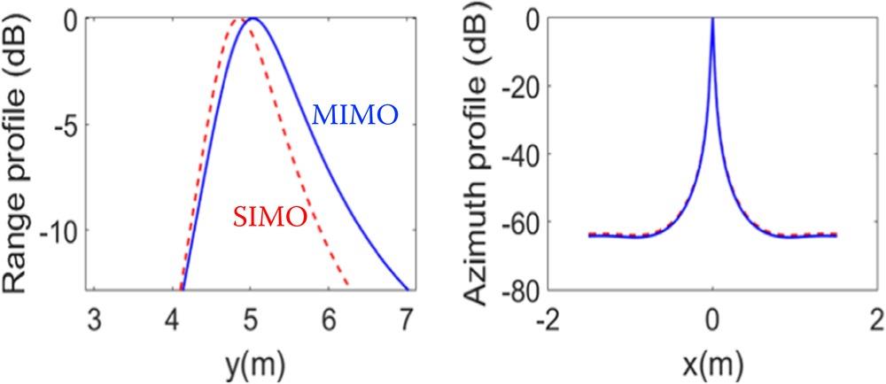
**FIGURE 8.2** Comparison of space-frequency TR-MUSIC imaging target in free-space by SIMO and MIMO: range profile and azimuth profile. The noise level was set to 0 dB.

For the imaging of a target in a random medium background, assuming that the target is an isotropic scatterer with a constant scattering amplitude, with the imaging scene shown in Figure 1.6. For N elements of TR array, we have a transmission matrix:

$⟨ K ⟩ = ⟨ σ_{s} g g^{Τ} ⟩$ (8.57)

where $⟨ ⟩$ is the ensemble average; $σ_{s}$ is the scattering coefficient, T denotes the matrix transpose, and

$g = {[G (R_{1}, X_{p}, w), G (R_{2}, X_{p}, w), .. ., G (R_{N}, X_{p}, w)]}^{Τ}$ (8.58)

The matrix element of K is the transmission function between element i and element j given by a random Green’s function as:

$K_{i j} = σ_{s} G (R_{j}, X_{p}) G (X_{p}, R_{i})$ (8.59)

Then the Decomposition of the Time Reversal Operator (DORT) T is

$⟨ T ⟩ = ⟨ K K^{†} ⟩$ (8.60)

where $†$ denotes the conjugate transpose operator, and the elements of T are

$⟨ T_{m n} ⟩ = \sum_{i = 1}^{N} ⟨ G_{m}^{*} G_{n} G_{i} G_{i}^{*} ⟩$ (8.61)

For the strong and weak fluctuations of the wave propagation in a random media, the circular complex Gaussian approximation imposes constraints. Assuming the circular complex Gaussian distribution, the fourth-order moment appearing in Equation (8.61) can be approximated from the second-order moment [25]:

$⟨ G_{m}^{*} G_{n} G_{i} G_{i}^{*} ⟩ = ⟨ G_{m}^{*} G_{n} ⟩ ⟨ G_{i} G_{i}^{*} ⟩ + ⟨ G_{m}^{*} G_{i} ⟩ ⟨ G_{n} G_{i}^{*} ⟩ - ⟨ G_{m}^{*} ⟩ ⟨ G_{n} ⟩ ⟨ G_{i} ⟩ ⟨ G_{i}^{*} ⟩$ (8.62)

The second order moment is recognized as a mutual coherence function:

$⟨ G_{i} G_{j}^{*} ⟩ = Γ_{i, j} (w_{1}, w_{2})$ (8.63)

Using the parabolic equation (PE) approximation, we have

$Γ_{i, j} = G_{i o} (w_{1}) G_{j o} (w_{2}) \exp (- Q_{i, j})$ (8.64)

where G_io is the free-space Green’s function:

$G_{i o} = - \frac{i}{4} H_{0}^{(1)} (k_{1} | R_{i} - X_{p} |), k_{1} = \frac{w_{1}}{c}$ (8.65)

where $H_{0}^{(1)}$ is 0-order Hankle function of first kind. The factor $e x p (- Q_{i, j})$ accouts for random medium contribution. One possible solution is given in [26].

Now, the K matrix in full data (MIMO) space-frequency TR-MUSIC writes

$K (w_{m}) = [\begin{array}{l} k_{1 n} (w_{m}) \\ k_{2 n} (w_{m}) \\ .. . \\ k_{N n} (w_{m}) \end{array}] = [\begin{array}{l} k_{11} (w_{m}) & k_{12} (w_{m}) & .. . & k_{1 N} (w_{m}) \\ k_{21} (w_{m}) & k_{22} (w_{m}) & .. . & k_{2 N} (w_{m}) \\ .. . & .. . & .. . & .. . \\ k_{N 1} (w_{m}) & k_{N 2} (w_{m}) & .. . & k_{N N} (w_{m}) \end{array}], m = 1, . .. M$ (8.66)

and

$T (w) = [\begin{matrix} t_{1 n} (w_{1}) & t_{1 n} (w_{2}) & .. . & t_{1 n} (w_{M}) \\ t_{2 n} (w_{1}) & t_{2 n} (w_{2}) & .. . & t_{2 n} (w_{M}) \\ .. . & .. . & .. . & .. . \\ t_{N n} (w_{1}) & t_{N n} (w_{2}) & .. . & t_{N n} (w_{M}) \end{matrix}]$ (8.67)

where the elements are

$t_{i, j} (w) = [t_{i, j} (w_{1}), t_{i, j} (w_{2}) .. ., t_{i, j} (w_{M})] (i, j = 1, .. ., N)$ (8.68)

Following the same procedure in obtaining the imaging function of Equation 8.52 by singular value decomposition applying to Equation 8.67, we can readily perform TR-MUSIC imaging for target obscured by random medium. Table 8.1 gives the simulation parameters to compare the performance between the space-space and space-frequency TR-MUSIC. For imageing geometry, please refer to Figure 1.6.

TABLE 8.1
Simulation Parameters Setting of Space–Space and Space–Frequency TR-MUSIC Imaging

Parameters	Symbol	Value
Pulse duration	T	4 ns
Carrier frequency	f_c	3 GHz
Number of elements	N	11
Element spacing		0.05 m
Pixel spacing		0.025×0.025 m²
	d₁	1.2 m
Medium depth	d₂	1.3 m
	d₃	2.5 m
Target location	T1	T1(0 m, 5 m)
Albedo		0.1/0.5/1
Optical depth	OD	0.1/1/5

From Figure 8.3, we see that the anti-noise performance of the space-frequency TR-MUSIC is significantly better than that of the space-space TR-MUSIC. When the Gaussian white noise with a signal-to-noise ratio of −10 dB is added, the space-frequency TR-MUSIC has a position offset but imaging quality is retained to a good level; by space-space TR-MUSIC the image is seriously defocused. As the signal-to-noise ratio increases to 0 dB, the space-space TR-MUSIC still cannot achieve the imaging of the target, but the space-frequency TR-MUSIC imaging is improved significantly, and the fact is more so when the signal-to-noise ratio continues to increase. Figure 8.4 shows the profile cuts of the target image T1 under different signal-to-noise ratio levels. From the figure, it can be seen that the azimuth resolution is better than the range resolution by both methods, with space-frequency TR-MUSIC being superior to the space-space TR-MUSIC. It is also clear that the stronger the noise, the greater the range displacement in the space-space TR-MUSIC.

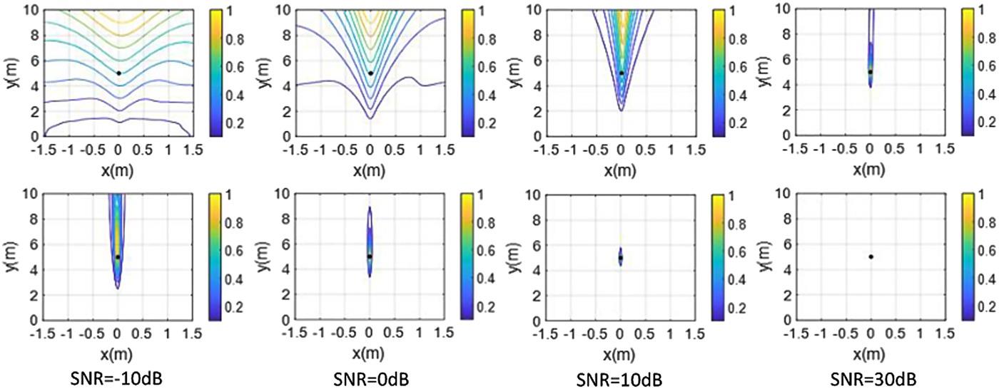
**FIGURE 8.3** Comparison of imaging results under different noise levels: top row: space-space TR-MUSIC; bottom row: space-frequency TR-MUSIC.

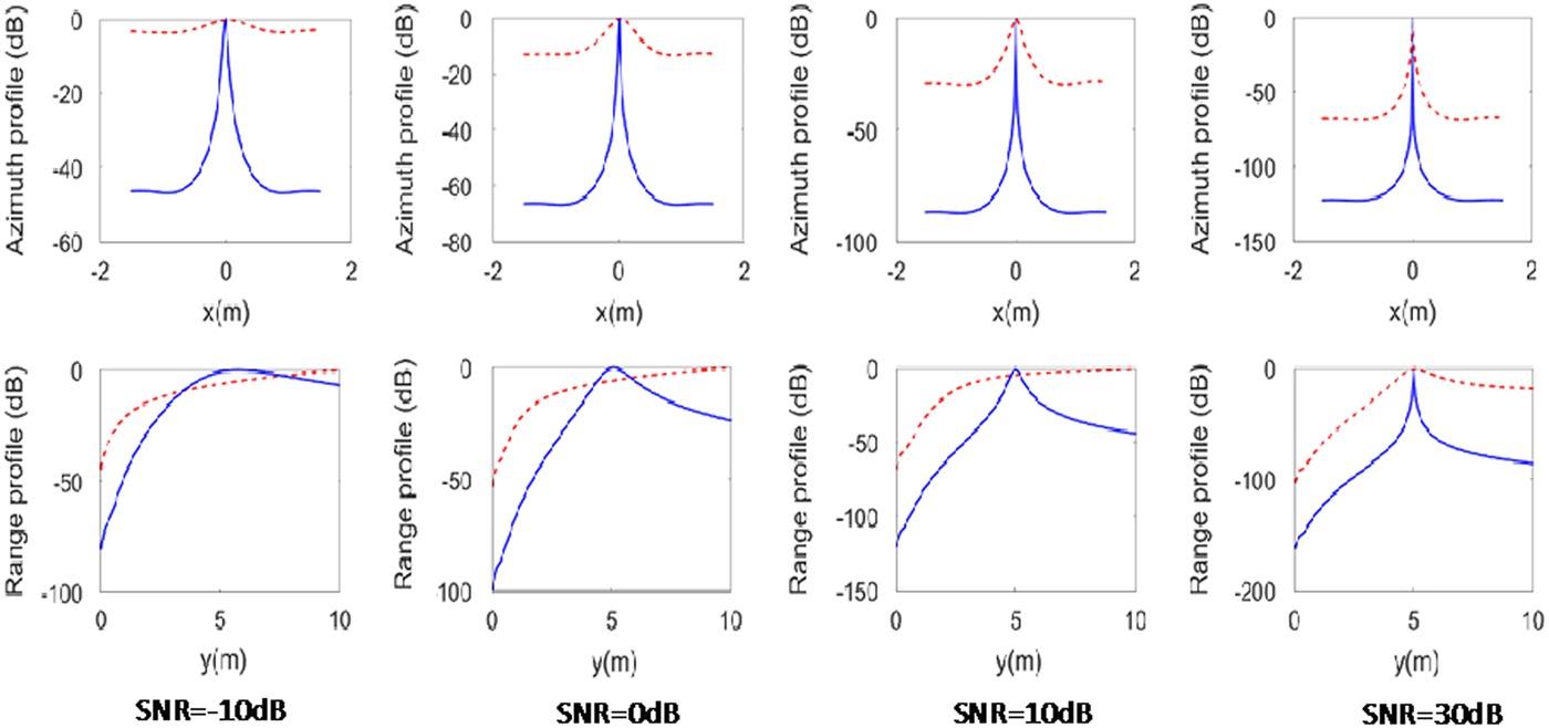
**FIGURE 8.4** Comparison of space-space TR-MUSIC (red dash-line) and space-frequency TR-MUSIC (blue-line) imaging resolution under different signal to noise levels.

Now, we examine the random media effect on the imaging performance. Figure 8.5 shows the target imaging results under different random media background. When OD = 0.1 and Albedo = 0.1, the space-space TR-MUSIC can achieve accurate imaging of the target; with the increase of the single scattering albedo, although the imaging results appear defocused in the longitudinal direction, the target can still be achieved Imaging. When OD = 1 and Albedo = 0.1, the imaging of the target can be achieved. However, with the increase of optical thickness and the increase of single scattering albedo, the traditional space-space TR-MUSIC cannot achieve focused imaging of the target. It can be seen that when OD = 0.1, it means that the random medium has less influence and is close to free space. When OD = 5, it means that the influence of random media is greater. The greater the optical thickness, the greater the single-scatter albedo, indicating that the random media has a greater impact on the target imaging.

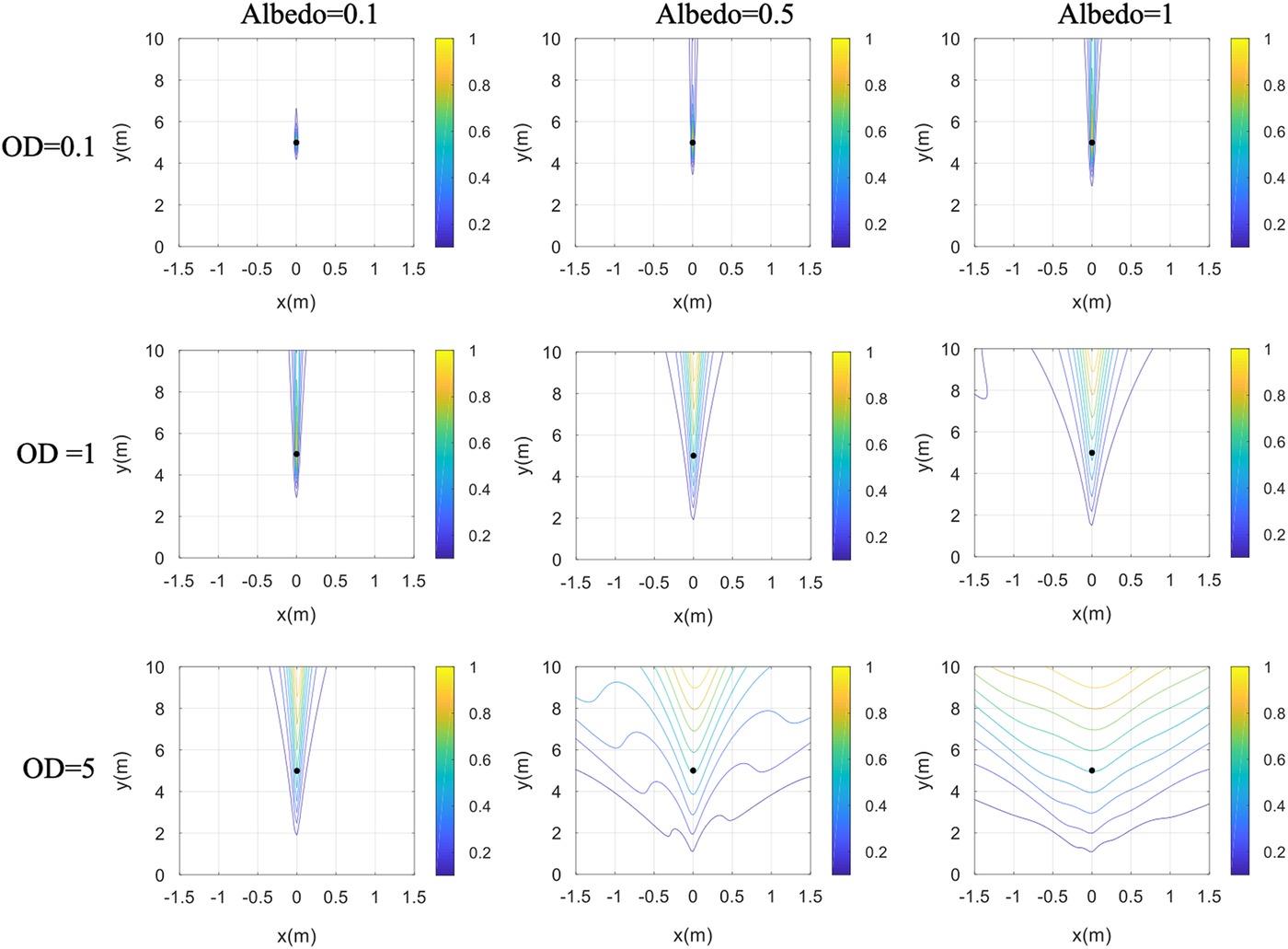
**FIGURE 8.5** Space-space TR-MUSIC imagining results under different parameters of random media (f_c=3 GHz).

Similarly, we examine the imaging performance of space-frequency TR-MUSIC under the influence of a random medium. It can be seen from Figure 8.6 that when the OD is 0.1, although with the increase of Albedo, the image point becomes larger and the focusing effect becomes worse. But compared with the space-space TR-MUSIC, its change is smaller. When OD = 1, with the increase of Albedo, the vertical focusing performance of the image becomes significantly worse. When OD = 5, albedo = 0.5, and 1, the space-frequency TR-MUSIC has a serious defocusing phenomenon in both azimuth direction and range direction; its imaging performance is still superior to the space-space TR-MUSIC.

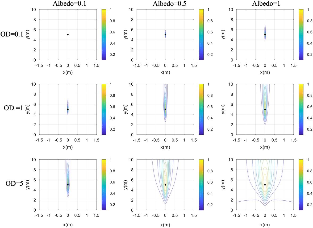
**FIGURE 8.6** Space-frequency TR-MUSIC imagining results under different parameters of random media (f_c = 3 GHz).

To further verify the space-frequency TR-MUSIC, the imaging performance with the same set of parameters but at a carrier frequency of 24 GHz is shown in Figure 8.7. Comparing it with Figure 8.6 shows that when OD = 0.1, 1, the effect of the random media is weak. As the frequency increases, the wavelength becomes shorter, and the penetration through the random medium is shallower, resulting in a significant deterioration of the distance resolution; when OD = 5, Albedo = 1, the influence of the random medium is stronger and further deteriorates the imaging performance.

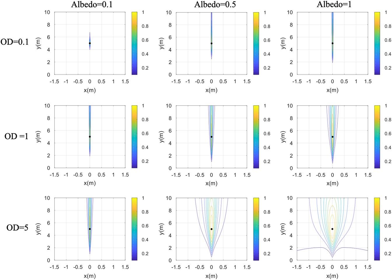
**FIGURE 8.7** Same as Figure 8.6 but at f_c = 24 GHz.

A short remark about the imaging performance of TR-MUSIC may be drawn at this point. From the above simulations, both optical thickness and single-scatter albedo are the two main factors that affect the target imaging performance in the presence of random media. Compared to azimuth resolution, range resolution is deteriorated to a greater extent by random media. When the scattering thickness is large, the wave propagation is more affected by the random medium, and more energy is scattered, so that the influence from the random medium is enhanced, resulting in a poor target imaging.

8.3 SYNTHETIC APERTURE IMAGING

8.3.1 SIGNAL MODEL

SAR echo signal in the time domain is a result of scattered field $E_{s_{τ}} (τ, η)$ , also called the reflectivity field, convolving with the radar system impulse response, or point spread function, $P S F_{τ} (τ, η)$ , and is mathematically expressed as, assuming a pulse radar:

$\begin{array}{l} s_{0} (τ, η) & = & E_{s_{τ}} (τ, η) \otimes P S F_{τ} (τ, η) \\ = & E_{s_{τ}} (τ, η) \otimes \\ [p_{r} (τ - \frac{2 R (η)}{c}) g_{a} (η - η_{c}) \exp {- j 4 π f_{c} \frac{R (η)}{c}} \exp {j π a_{r} {[τ - \frac{2 R (η)}{c}]}^{2}}] \end{array}$ (8.69)

where $τ, η$ represent the fast time and slow time, respectively; $\otimes$ is convolution operator in the time domain; $R_{c}$ is the SAR range to the center of footprint and varies with the slow time; $a_{r}$ is the chirp rate, $f_{c}$ is the carrier frequency.

In Equation 8.69, $p_{r}$ is a pulse waveform, and $g_{a}$ denotes the azimuthal antenna pattern with a typical form:

$\begin{array}{r} g_{a} (η - η_{c}) ≅ {sinc}^{2} {\frac{0.886 \cdot θ_{d i f f} (η - η_{c})}{θ_{a z}}} \end{array}$ (8.70)

where $θ_{d i f f}$ denotes the angle difference between beam center and instantaneous target angle; $θ_{a z}$ is the antenna beamwidth at azimuthal direction; $η_{c}$ stands for the azimuth crossing time at azimuth beam center.

Equivalently, the echo signal at frequency domain with linear frequency modulation in the chirp signal can be given by taking the Fourier transform of Equation 8.69 in fast time $τ$ as:

$S_{0} (f_{τ}, η) = E_{s_{f}} (f_{τ}, η) \times P S F_{f_{τ}} (f_{τ}, η) = E_{s_{f}} (f_{τ}, η) \times [P_{r} (f_{τ}) g_{a} (η - η_{c}) \times \exp {- j \frac{4 π (f_{c} + f_{τ}) R (η)}{c}} \exp {- j π \frac{f_{τ}^{2}}{a_{r}}}]$ (8.71)

As for estimating the scattered field from the imaging target, be it distributed or single, there exist numerous fast computational algorithms [27]. For the purpose of demonstration, the ray-tracing approach, combining with the ray tracing, the Physical Optics (PO) and Physical Theory of Diffraction (PTD) methods [22] is given. As we stated in the last section, estimation of the scattered field in the time of SAR transmitting the incident signal toward the target can be by full-wave solution or the approximate solution such as Born, Rytov, PE approximations, among other choices, as discussed previously. In approximate solution, for the more complex targets, the high order Taylor expansion is preferable for solving the surface current density over which the scattered field is obtained by integration, so that the multiple scattering is taken into account. Furthermore, an analytical diffraction solution is applied to the wedge structure that is very common in geometrically complex targets. Accounting for the multiple scattering or bounces, Equation 8.71 can be rewritten as a coherent sum of the individual bounce ( $m = 1, 2, .. . M_{b}$ ):

$S_{0} (f_{τ}, η) = \sum_{m = 1}^{M_{b}} {\vec{E}}_{s_{f}} (f_{τ}, η) \times [P_{r} (f_{τ}) g_{a} (η - η_{c}) \times \exp {- j \frac{4 π (f_{0} + f_{τ}) R_{m} (η)}{c}} \exp {- j π \frac{f_{τ}^{2}}{a_{r}}}]$ (8.72)

where R_m is the slant range of the m^th bounce; ${\vec{E}}_{s_{f}}$ is scattered field in frequency domain. When simulating the echo signal, either Equation 8.69 or Equation 8.71 can be applied, at least mathematically. Computationally, it is not so, as can be seen from the comparison between time domain and frequency domain given in Table 8.2, where M denotes the grid number at azimuth; N is the range bin number; P is the discrete sample of reflectivity map in single azimuth line; Q is the convolution kernel size that is with regard to the chirp signal, and R is the number of bouncing. Note that the ray tracing is desirable in both time and frequency domains.

TABLE 8.2
Comparison of Time and Frequency Domain for a Single Range Bin

Item	Time Domain	Frequency Domain
Multi-bounce	Finding the bouncing numbers with mesh grid, T = M	Finding the bouncing number with mesh grid, T = M
Multi-level combination	Merging the reflectivity fields for all of complex target, T = R	—
Convolution	2D convolution with reflectivity map, T = (PQ)log₂(PQ)	—
Multiplication	—	Pixel-wise multiplication for each bouncing level, T = MNR
Time complexity	O(n²log₂n²)	O(n²)

In the time domain, it requires to compute the convolution for each azimuth line with scattered field (reflectivity field) within the area of instantaneous footprint at certain azimuth slow time. Based on the fast Fourier transformation, the time complexity can be reduced to O(log₂(P+Q)) and for all of the azimuth positions, M, can be extended to O(M(P+Q) log₂(P+Q)). Indeed, the multi-bounce is hidden in the pre-processing using the reflectivity field combination. On the other hand, in the frequency domain, we only need to consider the pixel-wise multiplication and the multi-bouncing, and the time complexity is O(MNR). To this end, it is clear that SAR echo signal simulation in the frequency domain is a better choice [28].

8.3.2 SAR PATH TRAJECTORY

For a more realistic echo simulation, SAR’s path trajectory that perturbs the Doppler estimation must be considered. For tracking the SAR moving path, a series of coordinates transformations are necessary. The geo-location with longitude/latitude/height (LLH) coordinate, known as Geocentric coordinate is attained to produce the geo-reference SAR image, which can be projected onto the ground map. As for SAR’s attitudes, pitch/roll/yaw (PRY) coordinate, which generates the squint angle, and determines the antenna pointing vector and the antenna pattern [29]. For example, the pitch angle induces the squint angle that subsequently changes the Doppler centroid. The vibration of the SAR motion also gives rise to bias and noise attached to the attitudes within the path trajectory tunnel, where, the bias is measurable, while the noise is immeasurable. In order to simulate these vibration effects, the coordinate transformations between the SAR observation geometry and the local geometry must be included.

As far as the path trajectory is concerned, one must consider the state vector including the position $[X, Y, Z]$ , the tangential velocity $[V_{x}, V_{y}, V_{z}]$ , and the attitude $[α, β, γ]$ , all of them must be recorded as the sensor parameters. The basic idea of relationship of each coordinate is below. First of all, we need to define the SAR movement.

From the SAR observation geometry in Figure 8.8, it is known that the slant range $R (η)$ varies along the slow time $η$ . Ideally, it can be rewritten as

$\begin{array}{r} R (η) = \sqrt{R_{0}^{2} + {(v η - v η_{0})}^{2}} \approx R_{0} + \frac{{(v η - v η_{0})}^{2}}{2 R_{0}} \end{array}$ (8.73)

where $η_{0}$ corresponds to R₀, the shortest range. Indeed, $R (η)$ may be seen as a measurable slant range under the vibration- free motion. In reality, there is no vibration-free motion, where the slant range becomes $R' (η)$ , which now can be expressed in Line-of-sight (LOS)/parallel/perpendicular (LPP) coordinate [28,29]:

$\begin{array}{l} R' (η) & = & \sqrt{{(R_{0} - d_{L O S} (η, r))}^{2} + {(v η - v t_{0})}^{2} + d_{⊥}^{2} (η)} \\ \approx R_{0} + \frac{{(v η - v η_{0})}^{2}}{2 R_{0}} - d_{L O S} (η, r) + \frac{d_{L O S} η (η, r)}{2 R_{0}^{2}} {(v η - v η_{0})}^{2} \\ + \frac{d_{⊥}^{2} (η)}{2 R_{0}} + \frac{d_{L O S} (η, r)}{2 R_{0}^{2}} d_{⊥}^{2} (η) \\ ≜ R (η) + Δ R \end{array}$ (8.74)

where $d_{L O S}$ is the distance along the line of sight, and $d_{⊥}$ is the cross product of d_|| and $d_{L O S}$ , with d_|| being the distance along the instantaneous tangential velocity direction [29].

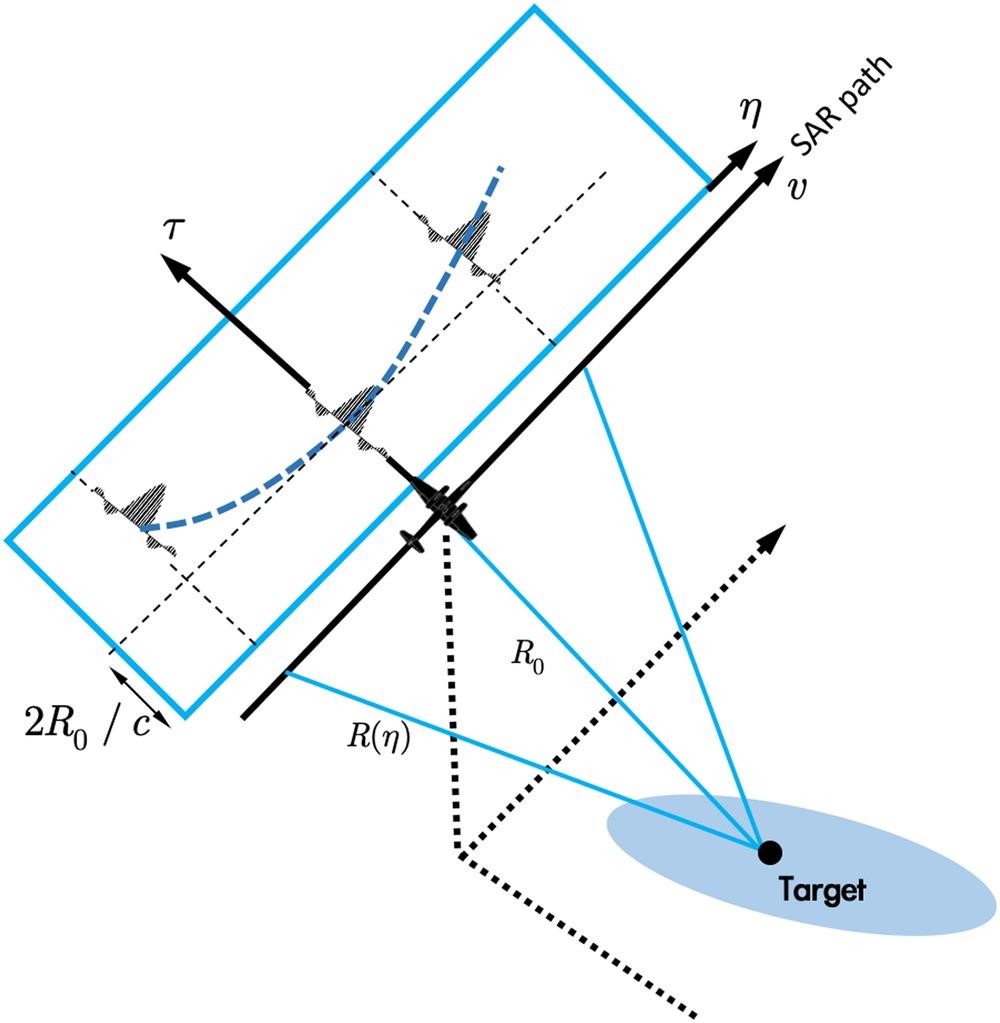
**FIGURE 8.8** A side-looking strip map SAR observation geometry in slow-fast time coordinate.

The differential slant range, $Δ R$ , in Equation 8.74 is given by:

$Δ R = - d_{L O S} (η, r) + \frac{d_{L O S} (η, r)}{2 r^{2}} {(v η - v η_{0})}^{2} + \frac{d_{⊥}^{2} (η, r)}{2 r} + \frac{d_{L O S} (η, r)}{2 r^{2}} d_{⊥}^{2} (η, r)$ (8.75)

where the first two terms on the right-hand side are influenced by $d_{L O S}$ , the third term is determined by $d_{⊥}$ , and the last term is the coupling term, the higher-order term.

The ENU coordinate representing the local position in east/north/up directions, respectively, can be expressed in the LLH coordinate with $[ϕ, θ, h]$ denoting the longitude, attitude, and height, respectively [28,29]:

$P_{e n u} = [\begin{matrix} x_{e} \\ y_{n} \\ z_{u} \end{matrix}] = [\begin{matrix} (φ - φ_{0}) (E_{b} + h) \cos θ \\ (θ - θ_{0}) (E_{a} + h) \\ h - h_{0} \end{matrix}]$ (8.76)

where $[θ_{0}, ϕ_{0}, h_{0}]$ denotes the origin position; $E_{a}$ and $E_{b}$ are the semi-major and semi-minor axis length of earth. With the transformation matrices, $M_{1}$ and $M_{2}$ given in[19], the ENU coordinate can be transformed to the LPP coordinate:

$P_{d} = {[d_{L O S}, d_{∥}, d_{⊥}]}^{T} = M_{2} M_{1} P_{e n u}$ (8.77)

where $[d_{L O S}, d_{∥}, d_{⊥}]$ is in LPP coordinate. The noisy position and velocity can be initialized within the $d_{⊥}$ and $d_{L O S}$ . It follows that to take into account the path trajectory, the SAR’s state vector, $P_{e n u}$ , can be derived from Equation 8.76.

8.3.3 ANTENNA BEAM TRACKING

In SAR image simulation, both radiometric and geometric fidelities must be preserved as much as possible. In the radiometric aspect, when computing the scattered field from a target being imaged, we must consider the azimuth antenna angle, defined in Figure 8.9, where $η_{c}$ is the center azimuth position, and $η_{1}$ , $η_{2}$ denote the initial and final positions of SAR, respectively, within the course of synthetic aperture. For arbitrary antenna pointing direction, Φ measures the azimuth angle covering the target region in a single footprint, while he angle Φ’ represents the azimuth angle from the antenna beam center to target’s center. It should be noted that in ray tracing, we have to deal with multiple rays within an illuminated target.

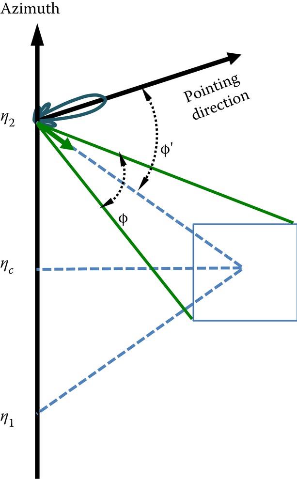
**FIGURE 8.9** The azimuth antenna angle with respect to the SAR moving and looking the target within the course of synthetic aperture.

In Circle and Spotlight SAR data acquisition modes (see Figure 1.4), only a single footprint is involved because the region of observation is limited to be within a footprint. But it is not so in Stripmap mode, which uses push broom to obtain a wider range of data taken in the azimuth direction. To be more realistic in simulation, modifications are needed for Stripmap mode. As the SAR moves, at arbitrary azimuth position, the azimuthal antenna scanning angle is bounded by [28]:

$\begin{array}{r} Φ_{scan}^{i} = \min (Φ_{3 dB}^{i}, Φ_{target}^{i}), i \in [azimuth, range] \end{array}$ (8.78)

where $Φ_{3 d B}^{i}$ and $Φ_{t a r g e t}^{i}$ are the covering angles of antenna 3 dB beam-width and target, respectively, and need to be estimated for computing the scattered filed. Notice that $Φ_{s c a n}^{i}$ is also affected by the squint angle effect, $θ_{s q}$ . Similarly, the covering angles should be estimated along the slant range, so that the image simulation can be feasible for the arbitrary size of the target.

8.3.4 SIMULATION EXAMPLES

Referring to Figure 8.8, suppose that the SAR system moves along the y-direction with ground range in x-direction. Then, the scattered field received by SAR traveling along the y-direction, at far-field range R, can be expressed as

$E_{s} (R, t, η) = \frac{e^{- j ω t} e^{- i k R}}{4 π R} \int J (r') e^{i k \cdot r'} e^{- \frac{{(x' - x_{c})}^{2} \cos^{2} θ_{s}}{R_{0}^{2} β^{2}}} e^{- \frac{{(y' - y_{c})}^{2}}{R_{0}^{2} β^{2}}} d S'$ (8.79)

where J(r′) are surface current density, with a two-dimensional Gaussian antenna gain pattern with full beamwidth β, centered at a resolution cell (x_c, y_c). In SAR, the received signal, called the echo signal, is a coherent sum of all scattered fields received at R:

$E_{s} (t, η) = \int_{0}^{L_{s}} E_{s} (t, R (η)) d y$ (8.80)

where L_s is the synthetic aperture length.

Noted that in transmitting signal and receiving signal, the wave polarizations can be chosen. After demodulation, the received signal of Equation 8.80 is then Fourier transformed and is ready for image focusing processing. Figure 8.10 illustrates a functional block diagram of a SAR image simulation. The simulation processing flow is adopted from [28]. Generally, the inputs include the platform, radar parameter settings, and target computer-aided design (CAD) model. Then, the scattering fields are calculated within different platform positions, and the echo signal can be generated in two dimensions, followed by an imaging algorithm to achieve the final focused image. A refined omega-K algorithm was chosen to perform SAR image focusing [28,29].

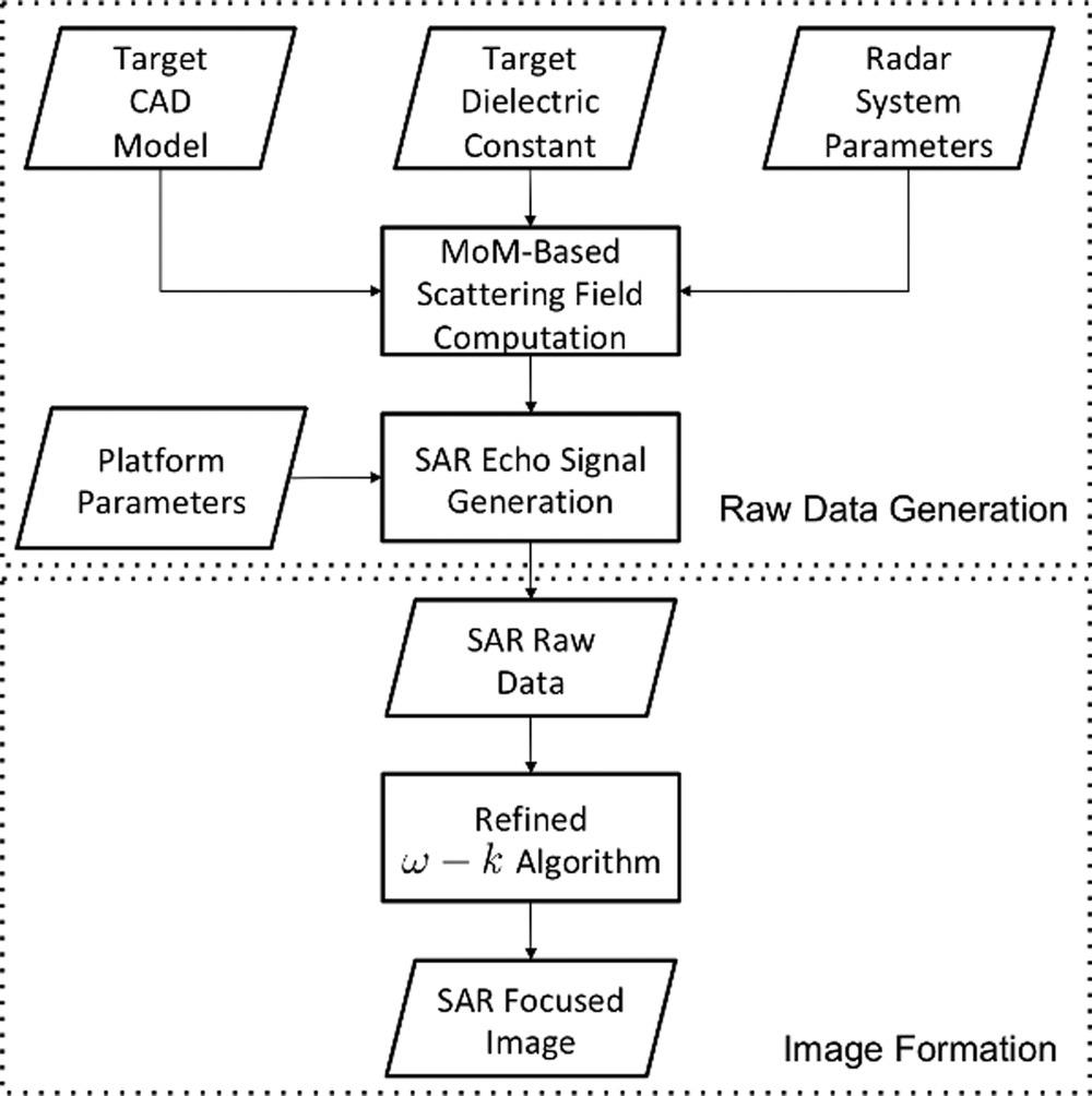
**FIGURE 8.10** A Full-wave based SAR image simulation flowchart.

The numerical simulations are based on a practical experimental configuration with a total synthetic length of 1 m and a maximum slant range of 1.8 m. The system height from the ground plane is 1.5 m with a look angle of 45°. The antenna beam width is from a typical standard gain horn antenna. The signal carrier frequency was set at 36.5 GHz with a 10 GHz bandwidth. Selected specifications are shown in Table 8.3. More details are given in [30].

TABLE 8.3
Simulation Parameters for a Full-Wave Based SAR

Parameter	Value	Unit
Carrier Freq.	36.5	GHz
Bandwidth	10	GHz
Sensor Height	1.5	m
Target Location	1.1	m
Sensor Position Interval	1	cm
Look Angle	45	degree
Synthetic Length	1	m
Antenna Beam Width	17.5	degree
Sphere Radius	1.5	cm
Azimuth Angle (Incident)	0	degree
Azimuth Angle (Scattering)	0 and 180	degree
Scattering Angle (Bistatic)	45	degree

Now, simulations of metal, dielectric, and coatings (metal coated with Teflon) for two targets are used. Two spheres were separated along the azimuth direction, with a spacing of 0 mm, 5 mm, 10 mm, 15 mm, 20 mm, and 25 mm. The focused images in Figure 8.11 present the interaction among the targets. The case of two metal spheres features not only the two targets but also their mutual effects. The interactions are stronger with smaller displacement spacing and become weaker as the spacing increases. Due to the effects of transmission, scattering, and multi-path interactions, the results show more complex imagery in the case of the dielectric object.

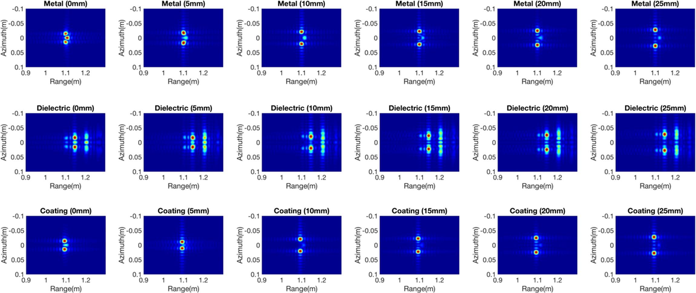
**FIGURE 8.11** Images of metal sphere, dielectric sphere, and metal sphere coated with Teflon with a spacing of 0 mm, 5 mm, 10 mm, 15 mm, 20 mm and 25 mm. (Top row: metal, middle row: dielectric and bottom row: metal coated with Teflon).

It is clear that multiple phase delays occur in the range direction, which includes the different levels of interactions with the spacing changes. In the case of coated spheres, only parts of the power is scattered back because of the presence of the inner metal sphere (see Figure 8.12), and the interaction is weaker. By testing different types of material, different degrees of interaction among targets can be analyzed in the simulations.

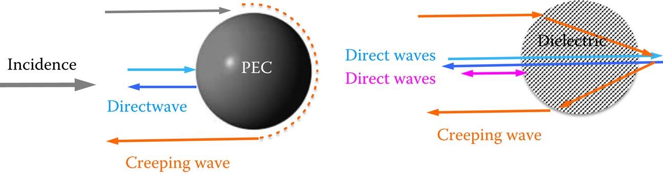
**FIGURE 8.12** Physical interpretation of multiple phase delays for PEC sphere (left) and dielectric sphere (right).

More complex target arrangements in Figure 8.13 are simulated in three dimensions by three spheres (both the metal and dielectric) placed both along the range and azimuth directions with no spacing in the scene center. In the case of multiple targets, the interactions are weaker in the range than in the azimuth direction. The different level of interactions in the azimuth direction is due to mutual effects among targets. The electromagnetic characteristics in the dielectric objects are more complex, and mutual interactions and self-interactions are shown at the same time. The different interaction degrees are illustrated that reduce target recognition ability. The results in Figure 8.13 highlight the difference between the point-target model and the full-wave method.

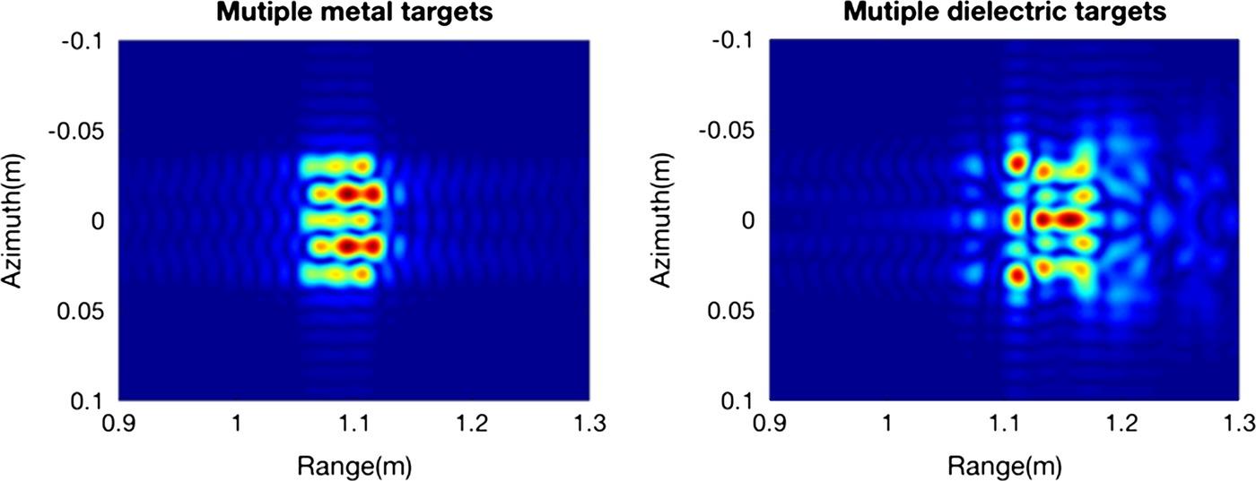
**FIGURE 8.13** Image of a cluster of three by three metal spheres (left) and dielectric spheres (right).

From the system aspect of the simulation, the system bandwidth is an important parameter in radar system design and is relative to the range resolution in the focused image. As the radar bandwidth increases, the electromagnetic interaction of a target can be resolved to varying degrees depending on the radar bandwidth. Hence, electromagnetic characteristics according to the variation in bandwidth in different materials are discussed. In the case of a single metal object, the radar bandwidth changes from 1 GHz to 10 GHz are shown in Figure 8.14. Because of single scattering behavior in a single metal target, the results show the bandwidth changing with little influence. Only the range resolution changes with the variation in bandwidth.

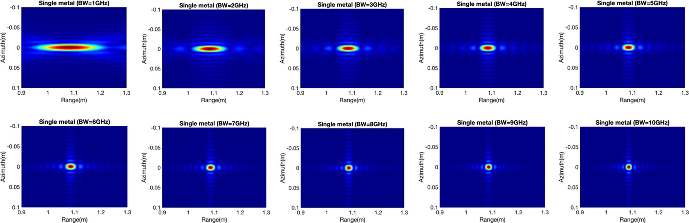
**FIGURE 8.14** Image of a metal sphere with SAR bandwidth varying from 1 to 10 GHz (from top to bottom).

Three different types of material (namely, Teflon, glazed ceramic, and GaAs) are used for analyzing the effect of bandwidth change for a single dielectric sphere. Due to the rich electromagnetic information in dielectric objects, the scattering effect based on system bandwidth is more pronounced. When the system bandwidth is small, the phenomenon of multiple scattering cannot be expressed because of the low range resolution. As the range resolution corresponds to the system bandwidth close to the size of the observation targets, the results show that one can make a distinction among different materials. When the system bandwidth reaches 5 GHz, that is, when the resolution is close to the object size level, the different target dielectric constants and the multiple scattering phenomena can be illustrated in the various levels of results. The focused images presented in Figure 8.15 demonstrate that system bandwidth is profoundly significant, as is well known, for imaging dielectric objects relative to the metal targets.

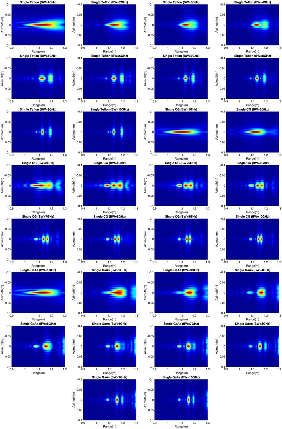
**FIGURE 8.15** Images of a dielectric sphere with SAR bandwidth varying from 1 to 10 GHz (top: Teflon; middle: glazed ceramic; bottom: GaAs).

The effect of the system bandwidth on two targets is also discussed. Two different kinds of metal and dielectric objects are simulated with no spacing between targets. As shown in Figure 8.16, when the system bandwidth is lower, the ability to differentiate between metal and dielectric objects is poor, but their mutual interaction can still be illustrated. Moreover, the bandwidth changes only affect the resolution variation because of electromagnetic wave nonpenetration for the two metal objects. On the other hand, bandwidth alternations strongly affect the multipath imaging of a dielectric material. Also, more complex objects are used for analysis of the system bandwidth. Both metal and dielectric materials with three-by-three spheres are placed along the range and azimuth directions with no spacing between objects. In the focused images of the metal spheres, the targets with mutual interaction in the azimuth direction can be identified, and the targets in the distance image cannot be recognized as three objects because of lower resolution in the range direction. As the system bandwidth increases, the mutual interactions in the different levels are presented with the corresponding resolution. For the dielectric materials shown in Figure 8.17, different degrees of electromagnetic interaction are delivered with the variation in system bandwidth.

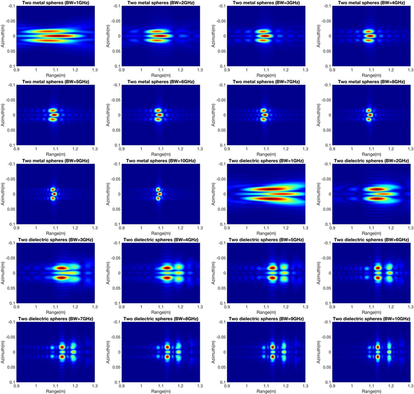
**FIGURE 8.16** Image of two metal spheres (top two rows) and two dielectric spheres (bottom two rows) with SAR bandwidth varying from 1 to 10 GHz.

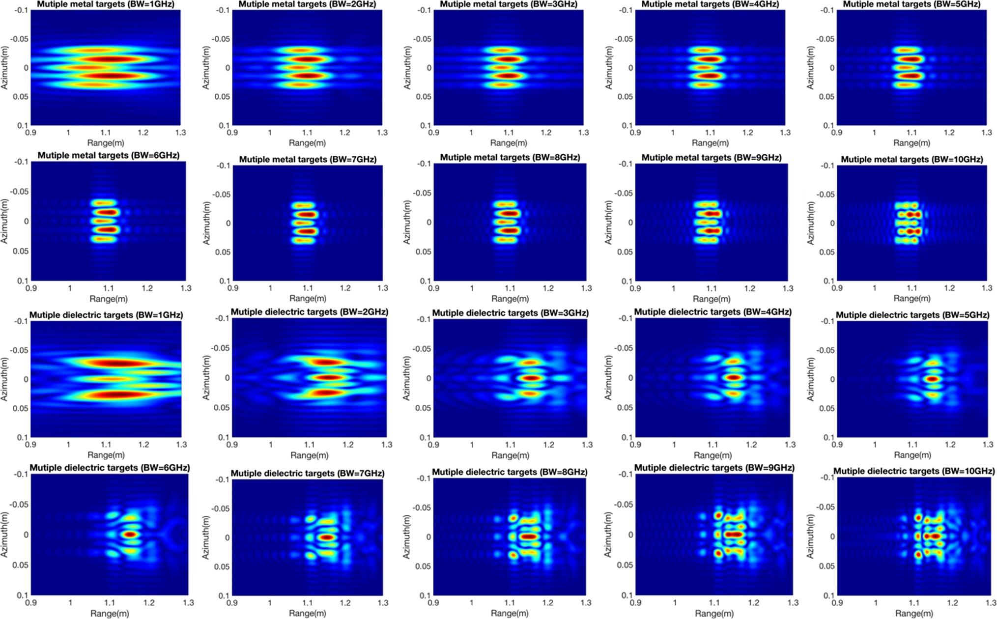
**FIGURE 8.17** Images of a cluster of multiple metal spheres (top two rows) and dielectric spheres (bottom two rows) with SAR bandwidth varying from 1 to 10 GHz.

We now present results of numerical simulation and experimental measurement. The experiments were set in an anechoic chamber and two metal spheres are placed in the scene center with spacings of 0 mm, 5 mm, 10 mm, 15 mm, 20 mm, and 25 mm. An N5224A PNA microwave network analyzer is used as a transmitter and receiver in this experiment. The system applied the motion controller to acquire data with a 1cm interval in the total 1 m synthetic length. After collecting the raw data, focusing is carried out to obtain the focused images. In Figure 8.18, the results from the full-wave method compare well with the experimental results. The approach preserves the electromagnetic wave interactions between two spheres, and the interaction is reduced with spacing increases. Various degrees of interactions are present with the spacing changes between the targets, and the interaction intensity is reduced with increasing spacing, as physically expected.

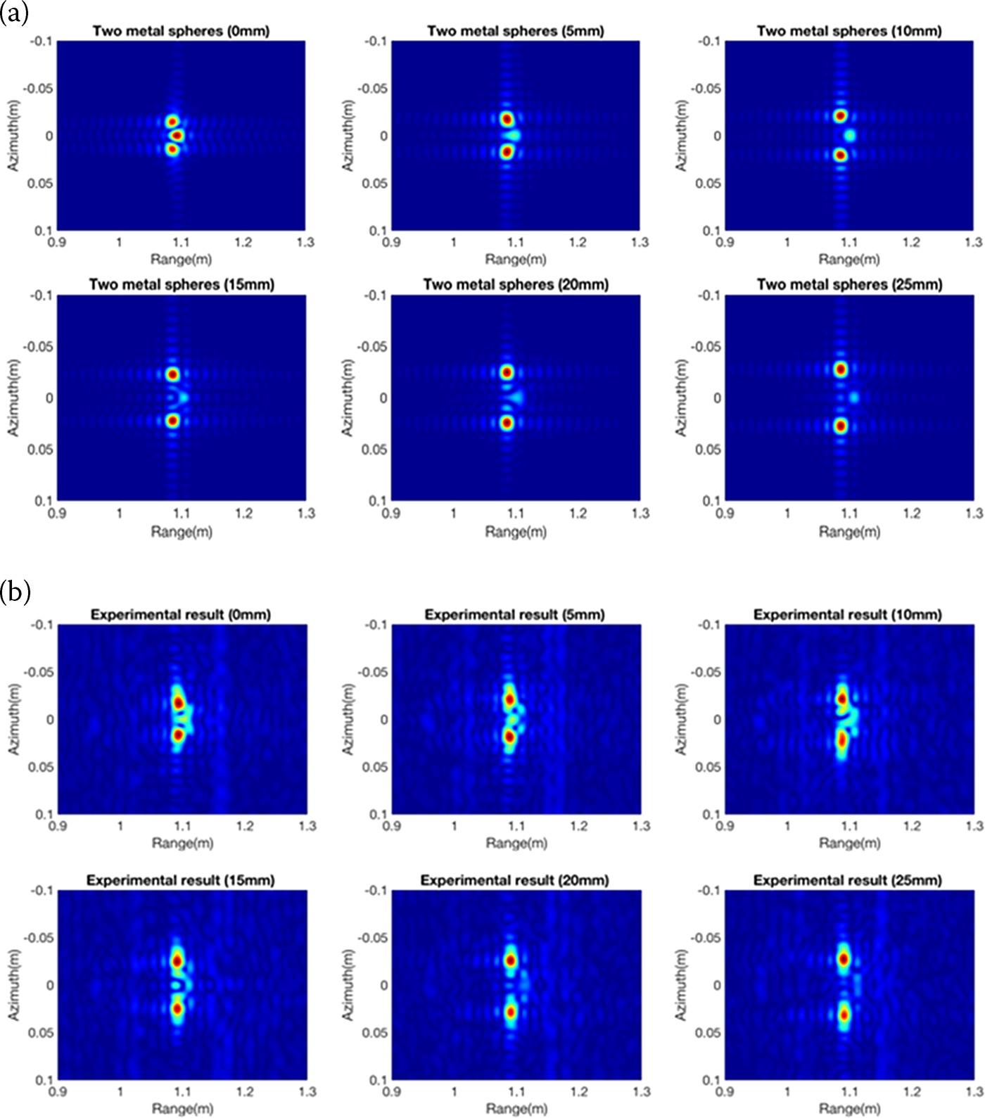
**FIGURE 8.18** Images of two metal spheres (top row: simulated; bottom row: experimental) with spacing of 0 mm, 5 mm, 10 mm, 15 mm, 20 mm, and 25 mm (from left to right).

8.4 MUTUAL COHERENCE FUNCTION

In acquiring the scattered field from the target, be it deterministic or random, we may devise it by forming diversity of mutual coherence function (MCF) in frequency, angular, space, polarization, etc. One such example is the coherency vector of radiated fields received by two antennas with displacement $\vec{d}$ given by [31]:

$V_{q p} (\vec{d}) = ⟨ E_{q}^{s} (\vec{r}) \otimes E_{p}^{s *} (\vec{r} + \vec{d}) ⟩$ (8.81)

where $⟨ ⟩$ is ensemble average; $\otimes$ is the outer product operator; * is a complex conjugate operator; p, q represents polarization. The polarimetric coherency vector in Equation 8.81 actually yields a compact expression that provides insight into interferometric SAR. By Cittert–Zernike theorem [32], the Fourier transform relationship of a brightness distribution with a polarimetric coherency vector can be established. A set of integral and differential equations for the correlation function of a wave in a random distribution of discrete scatterers [1]. Theses general integral and differential equations for spatial as well as temporal correlation function allow to observe the effects of the constant velocity as well as the fluctuating velocity. The MCFs for the scattered wave both for two frequencies and two scattering angles for one-dimensional rough surfaces were derived in [33–39]. The Kirchhoff approximation was used to obtain the scattered field. The scattering cross-section in the form of the two-frequency is available to conduct a series of simulation. The numerical calculation of the analytical results was compared with experimental data and Monte Carlo simulations showing good agreement. An analytic expression of the two-frequency mutual coherence function (MCF) was derived in [40] for a two-dimensional random rough surface. The scattered field was calculated by the Kirchhoff approximation. Their numerical simulations show that the two-frequency MCF is greatly dependent on the root-mean-square (RMS) height, while less dependent on the correlation length. Recalled that the first-order Kirchhoff approximation used in these papers does not include the effect of multiple scattering from different parts of the surface. Using the second-order Kirchhoff approximation (KA) with angular and propagation shadowing functions, the angular correlation function (ACF) of scattering amplitudes was developed to surfaces with large radii of curvature and high slopes of the order of unity [41]. An expression for the two-frequency mutual coherence function was also derived for studying waves propagating close to the ground, based on the parabolic wave equation model, which was solved by the path integral method [39]. The irregular surface height was assumed non-Gaussian distribution. Numerical schemes were developed for simulating the detection of buried objects embedded in rough surfaces [35–37].

For two-angle and two-frequency mutual coherence functions are formed by varying the transmitting or receiving angles or frequency, respectively (see Figure 8.19), and are mathematically given by

$V_{p q} (θ_{1}, θ_{2}) = ⟨ E_{p q}^{s} (θ_{1}) E_{p q}^{s *} (θ_{2}) ⟩$ (8.82)

$V_{p q} (f_{1}, f_{2}) = ⟨ E_{p q}^{s} (f_{1}) E_{p q}^{s *} (f_{2}) ⟩$ (8.83)

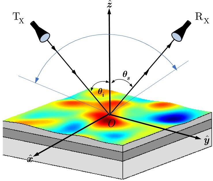
**FIGURE 8.19** Correlated scattered fields acquired at two angles or two frequencies.

In either way, the following baseline or memory line must be met:

$k_{1} \sin θ_{i 1} - k_{2} \sin θ_{i 2} = k_{1} \sin θ_{s 1} - k_{2} \sin θ_{s 2}$ (8.84)

where $k_{1}, k_{2}$ form two frequencies, and incident pair $θ_{i 1}, θ_{i 2}$ or scattered pair $θ_{s 1}, θ_{s 2}$ form the two angles.

As is noted, the polarizations p, q can be applied so that additional polarization diversity can be devised.

For the purpose of demonstration, we choose the following parameters: carrier frequency at 1.25 GHz, incident angles: 20° and 60°, surface roughness: kσ = 0.5λ, kl = 2λ, soil permittivity: $ε_{r} = 10 - j 0.05$ . We also set the incident and scattered azimuthal angles to 0°. To establish the mutual coherence functions in angle and frequency, the scattered angle varies from 90° to −90°, while the frequency increases a step of 0.01 GHz from a center frequency of 1.25 GHz and up to 2.25 GHz. Figures 8.20 displays the MCF on the angular-frequency plane at incident angles of 20^o. For all four polarizations, we see that the MCF responses bear quite a similar pattern, but the cross polarizations, HH and VH, have much small magnitude; perhaps it is due to the lack of sources for multiple scattering for this roughness scale. Figures 8.21 and 8.22 show the MCF responses to the soil moisture changes from 0.2 to 0.4. It indicates that the MCF is strongly dependent on the moisture content.

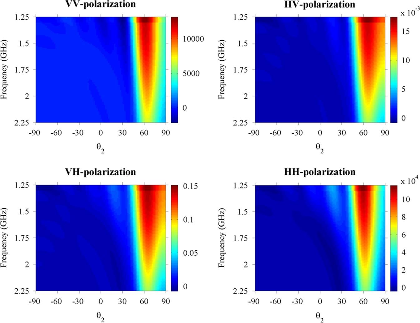
**FIGURE 8.20** Mutual coherence functions at four polarizations with 60° of incident angle.

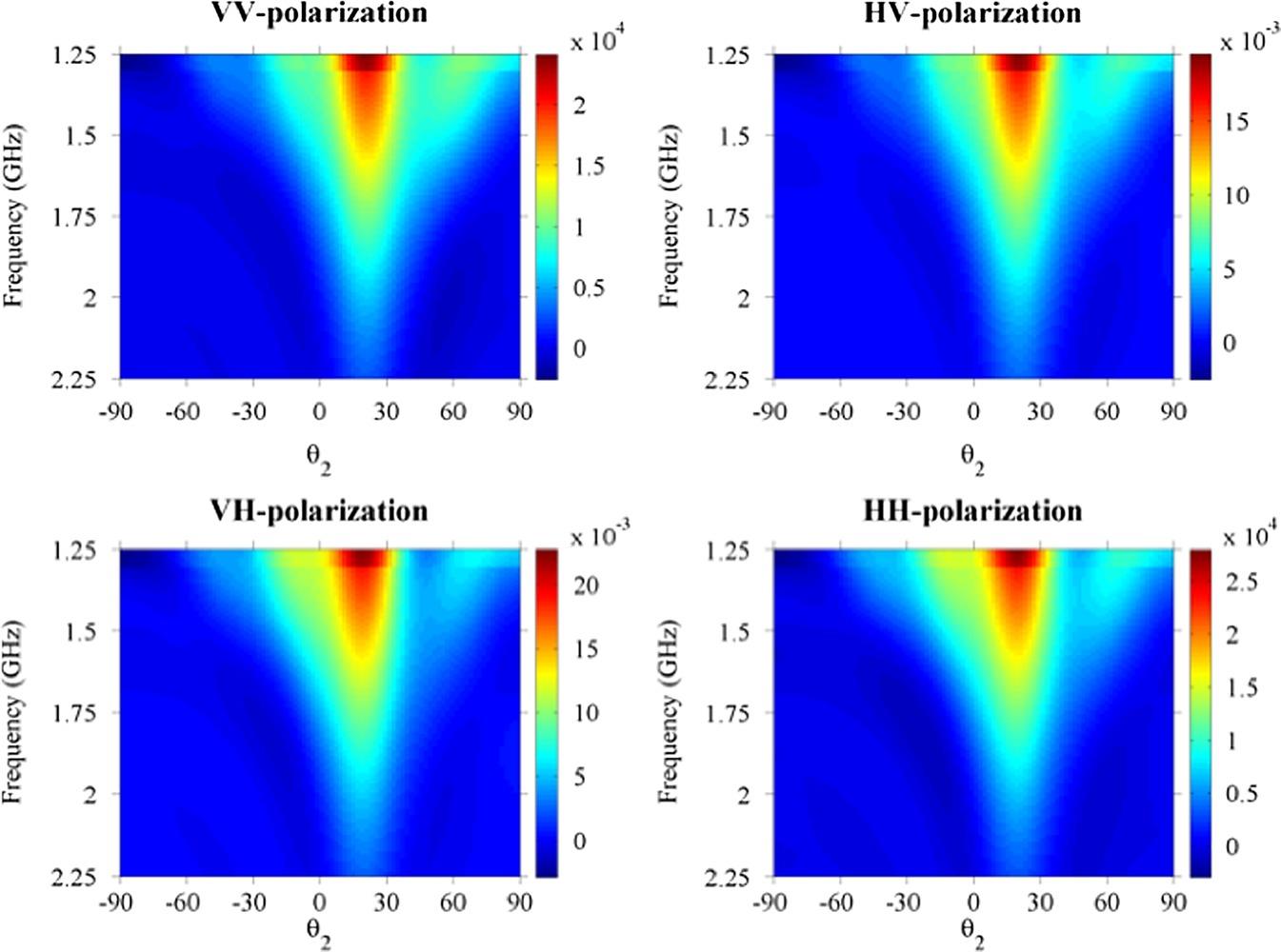
**FIGURE 8.21** Response of mutual coherence function to soil moisture: $m_{v} = 0.2$ .

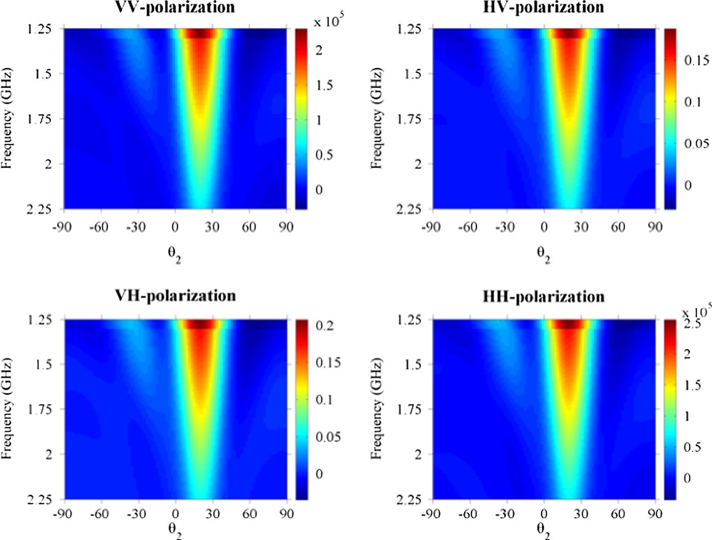
**FIGURE 8.22** Response of mutual coherence function to soil moisture: $m_{v} = 0.4$ .

8.5 BISTATIC SAR IMAGING

From Chapter 5, we have seen that bistatic scattering offers benefits of increasing the dynamic range of the returned signal strength and prompting higher sensitivity to the surface parameters. Hence it is demanded to acquire bistatic data. However, bistatic observation poses a high degree of freedom to configure the transmitter and receiver, to which each has elevation and azimuth angles to set. The topic itself covers a vast of subjects to explore. This subsection only discusses some basics in bistatic imaging, particularly in SAR.

8.5.1 BISTATIC SAR SCATTERING PROPERTY

A bistatic SAR imaging system separates the transmitter and receiver to achieve benefits such as exploitation of additional information contained in the bistatic reflectivity of targets, increased radar cross-section, and increased bistatic SAR data information content with regard to feature extraction and classification. Currently, similar to the monostatic SAR simulation, the point-target is used in bistatic SAR imaging, which is an efficient way to develop and compare algorithms. However, this approach is unable to achieve the advantages of bistatic SAR to extract target information in different aspect angles. Hence, to evaluate the proposed method, the results both in monostatic and bistatic mode are simulated for the special case of equal velocity vectors for the transmitter and receiver. Figure 8.23 presents the different scattering behavior under the same system parameters Table 8.3 with two directions of scattering azimuthal angles at 0° and 180°.

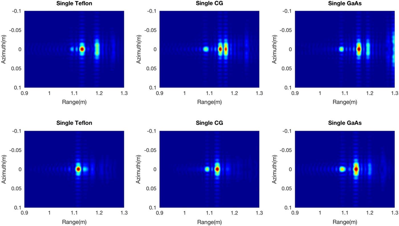
**FIGURE 8.23** Image of a single dielectric sphere for the monostatic versus bistatic (left: Teflon; center: ceramic glaze; right: GaAs). (top row: monostatic; bottom row: bistatic).

Using the same system parameters but with different observation angles, the intensity of the first bounce point in the bistatic results is the same as that in the monostatic: Increasing with increasing dielectric constant. However, the first bounce place moves backward in the bistatic simulation relative to the monostatic system. The effect of multiple scattering inside a sphere is significant in monostatic mode, but the behavior decays rapidly in bistatic mode. It is clear that the location of multiple scattering moves forward in the bistatic system [32].

Two targets in bistatic mode are also simulated with two spheres separated along the azimuth direction with spacing of 0 mm, 5 mm, 10 mm, 15 mm, 20 mm, and 25 mm. The look angle is 45° with azimuth angle at 0° and 180° in two observation modes. The results in Figure 8.24 show the interaction between two targets in both monostatic and bistatic observations; diversified scattering information can be obtained through different observation angles. For the simulation results of the two objects, the intensity of mutual interaction is lower in bistatic mode than monostatic. However, the intensity of creeping waves is enhanced in the bistatic simulation over the monostatic system.

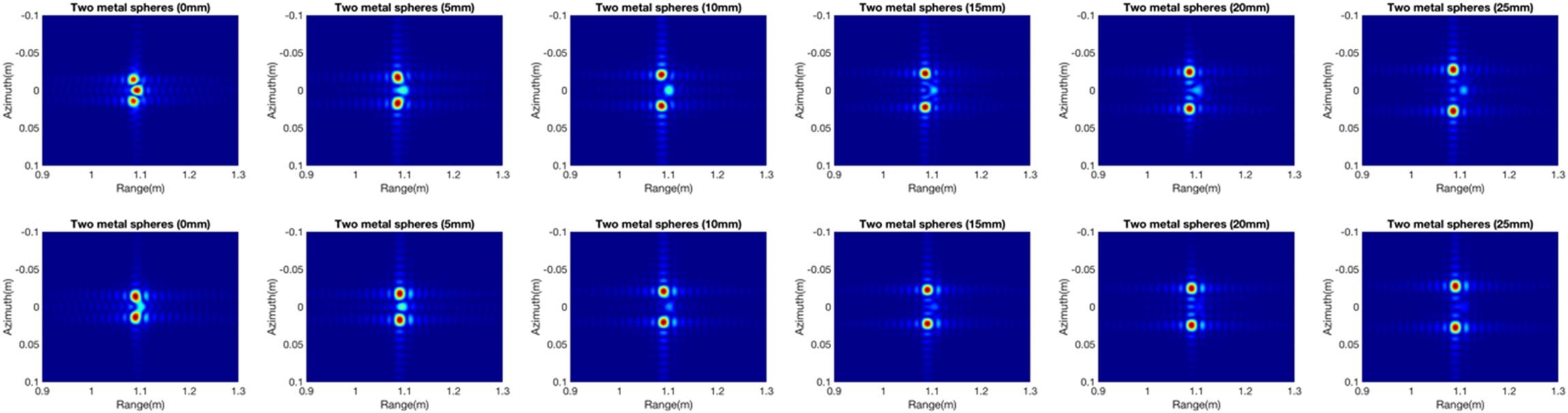
**FIGURE 8.24** Case simulations of two metal spheres in the monostatic and bistatic modes with spacing of 0 mm, 5 mm, 10 mm, 15 mm, 20 mm, and 25 mm (up: monostatic and bottom: bistatic).

Two-by-two metal targets placed along the range and azimuth directions are shown in monostatic and bistatic modes in Figure 8.25. Two spheres are set with no spacing in the azimuth direction, and another two are five wavelengths (0.0205 m) apart in the range direction. The monostatic case shows that original targets can still be identified with strong interaction in their centers. The interaction response is enhanced with the interaction in both the range and azimuth directions. As a result of the enhanced mutual interaction intensity, only the interaction is shown in the focused image, and the target recognition ability is reduced.

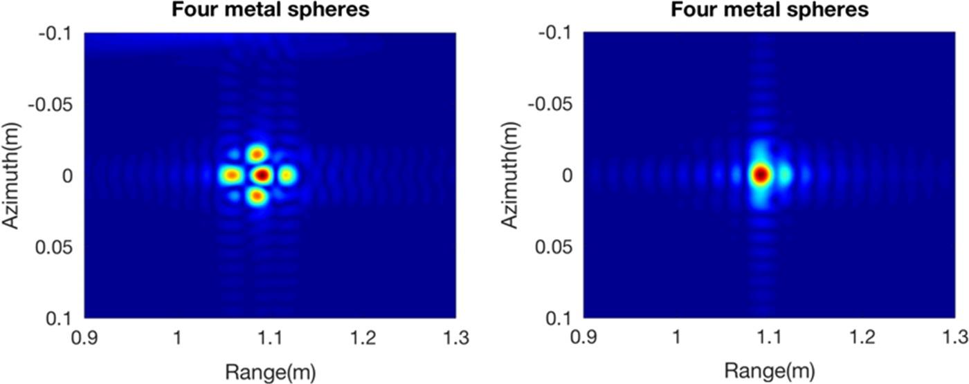
**FIGURE 8.25** Images of a cluster of two by two metal spheres in backward and forward modes (left: monostatic; right: bistatic).

Because of two separate carrier platforms, the performance analysis of the bistatic SAR imaging becomes more complicated than of monostatic SAR, in terms of bistatic range history, two-dimensional resolution, Doppler parameter estimation, and motion compensation and so on. In this chapter, we limit the evaluation of the bistatic range history and two-dimensional resolutions in the backward zone and in the forward incident plane zone.

8.5.2 BISTATIC IMAGING GEOMETRY AND SIGNAL MODEL

Now, we discuss the geometric property of backward and forward bistatic SAR based on the imaging geometry as depicted in Figure 8.26 [42]. In the imaging geometry, $θ_{T}$ and $φ_{T}$ are the incidence angle and transmitted azimuth angle and $φ_{R}$ the received incidence angle and received azimuth angle, with subscripts T and R denoting the transmitter and the receiver; the imaging space perhaps can be roughly divided into two zones, assuming a positive azimuth angle is counter-clockwise from the x-axis; the forward imaging zone is the area with the azimuth angle in the range of $φ_{R} \in (0 °, 90 °) \cup (270 °, 360 °)$ and another part belongs to the backward imaging zone. $P_{T} (η)$ and $P_{R} (η)$ are the instantaneous position vectors; V_T and V_R are the velocity vectors; $u_{T} (η)$ and $u_{R} (η)$ are the unit vectors in the direction from target P to the transmitter and receiver, respectively, at $η$ , with $w_{T} (η)$ and $w_{R} (η)$ denoting the angular velocities of the transmitter and receiver, respectively, at the time $η$ ; β is the velocity angle between the transmitter and the receiver velocity vectors. Notice that the monostatic backward imaging and bistatic forward specular imaging are located at $θ_{T} = θ_{R}, φ_{R} = 180 °$ and $θ_{T} = θ_{R}, φ_{R} = 0 °$ , respectively.

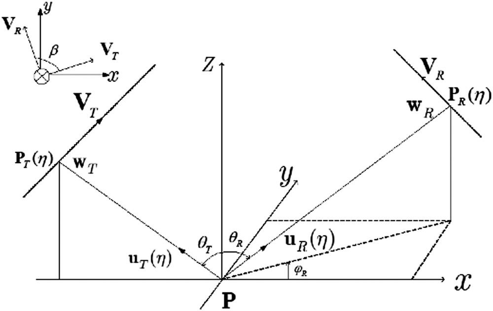
**FIGURE 8.26** Imaging geometry of bistatic SAR.

In the stripmap mode bistatic SAR, for analysis, some hypotheses are made in our study: first, we consider that the transmitter and the receiver sweep a continuous strip synchronously during the entire observation time, and second, the stop-and-go model is adopted. Finally, the ground plane of the imaging scenario is flat. If the curvature of the earth is considered, the whole scene can be divided into sub blocks so that the following analysis is still valid. Suppose that the transmitter sends a pulsed signal with duration time T_p and the carrier frequency f_c, defined as:

$s (τ) = w_{r} (τ) \exp [j (2 π f_{c} τ + π a_{r} τ^{2})]$ (8.85)

where $τ$ is the range time, a_r is the chirp rate and w_r is a rectangular gate function with width T_p. The demodulated baseband signal from a point target having a constant scatter amplitude A₀ is of the form

$s_{r} (τ, η) {= A}_{0} w_{r} (τ - \frac{2 R_{b i} (η)}{c}) w_{a} (η) \exp {(- j \frac{4 π f_{c} R_{b i} (η)}{c}) + j π a_{r} {(τ - \frac{2 R_{b i} (η)}{c})}^{2}}$ (8.86)

where c denotes the speed of light, $η$ is the cross-range time, $w_{a}$ is the antenna pattern in the cross-range direction and $R_{b i} (η)$ is the bistatic range, which is the sum of the ranges from the transmitter and the receiver to the target.

We now consider the two-dimensional ground resolution in a general configuration of bistatic SAR as shown in Figure 8.26. For the targets with a constant arrival time satisfy an iso-range surface $t (η) = \frac{‖ P_{T} (η) - P ‖ + ‖ P_{R} (η) - P ‖}{c}$ , upon projecting to the iso-range gradient vector, one can obtain the general form of the bistatic ground range resolution [43,44].

$ρ_{g r} = \frac{κ c}{B P_{z_{s}}^{⊥} u_{T} (η) + P_{z_{s}}^{⊥} u_{R} (η)}$ (8.87)

where $κ = 0.886$ when the antenna patterns and ranging waveform can be approximated by the rectangle pulse function; B is the signal bandwidth; $P_{Z_{s}}^{⊥}$ is the ground projection matrix given by

$P_{z_{s}}^{⊥} = [\begin{matrix} 1 & 0 & 0 \\ 0 & 1 & 0 \\ 0 & 0 & 0 \end{matrix}]$ (8.88)

and $u_{T} (η)$ and $u_{R} (η)$ are given by

$u_{T} (η) = \frac{P_{T} (η) - P}{P_{T} (η) - P}$ (8.89)

$u_{R} (η) = \frac{P_{R} (η) - P}{P_{R} (η) - P}$ (8.90)

Referring to Figure 8.26, for $P_{T} (η)$ , the main factors to determine the ground range resolution are the receiver motion parameters, including $θ_{R}$ and $φ_{R}$ . Based on the concept of the wavenumber vector or K-space, the bistatic azimuth resolution is calculated by

$ρ_{g a} = \frac{λ}{T_{a} (x, y) P_{z_{s}}^{⊥} w_{T} (η) + P_{z_{s}}^{⊥} w_{R} (η)}$ (8.91)

where the λ is the wavelength and $T_{a}$ is the synthetic aperture time of the target at $(x, y)$ ; $w_{T} (η)$ and $w_{R} (η)$ are the angular velocities of the transmitter and receiver, respectively, at the time $η$ , which are given by

$w_{T} (η) = \frac{[I - u_{T} (η) u_{T'} (η)] v_{T}}{P_{T} (η) - P}$ (8.92)

$w_{R} (η) = \frac{[I - u_{R} (η) u_{R'} (η)] v_{R}}{P_{R} (η) - P}$ (8.93)

with I the 3 × 3 identity matrix. If $P_{T} (η)$ and $v_{T}$ are known, for azimuth resolution, the main influences are the receiver motion parameters and the velocity angle, including $θ_{R}$ , $φ_{R}$ and β.

It is known that the ground range resolution and the azimuth resolution directions can be non-orthogonal in bistatic SAR mode [45]. From Figure 8.27, the resolution direction angle between the direction of the range gradient and that of the Doppler gradient can be calculated as

$ψ = accos (Θ \cdot Ξ)$ (8.94)

where $Θ$ and $Ξ$ are the unit direction vectors along the range resolution and azimuth resolution, respectively, given by

$Θ = \frac{P_{z_{s}}^{⊥} {(u_{T} (η) + u_{R} (η))}^{T}}{u_{T} (η) + u_{R} (η)}$ (8.95)

$Ξ = \frac{P_{z_{s}}^{⊥} {(w_{T} (η) + w_{R} (η))}^{T}}{w_{T} (η) + w_{R} (η)}$ (8.96)

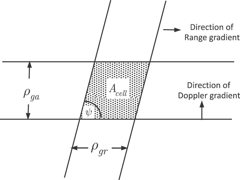
**FIGURE 8.27** The ground resolution cell of bistatic SAR.

The intercept imaging area of bistatic SAR is determined by the ground range resolution, the azimuth resolution, and the resolution direction angle, given by [43–45]

$A_{c e l l} = \frac{ρ_{g r} ρ_{g a}}{| \sin ψ |}$ (8.97)

8.5.3 BISTATIC RANGE HISTORY

An important difference in the forward bistatic SAR to that in the backward bistatic SAR is the existence of ghost effect, which will be explained by the range-history analysis as follows. At cross-range time $η$ , the bistatic range $R_{b i} (η)$ is the summarization of the distances of the transmitter and the receiver to the target $(x, y, z)$ :

$R_{b i} (η) = \sqrt{{(x - x_{T η})}^{2} + {(y - y_{T η})}^{2} + {(z - H)}^{2}} + \sqrt{{(x - x_{R η})}^{2} + {(y - y_{R η})}^{2} + {(z - H)}^{2}}$ (8.98)

It is clear that the iso-bistatic range $R_{b i} (η)$ surface in 3D space forms an ellipsoid with the transmitter and receiver at two foci. As the baseline between the transmitter and receiver decreases, the ellipsoid surface approaches a spherical surface. The intersection curve of the iso-bistatic range $R_{b i} (η)$ surface with the ground can be written as, setting $z = 0$ :

$R_{b i} (η) = \sqrt{{(x - x_{T η})}^{2} + {(y - y_{T η})}^{2} + H^{2}} + \sqrt{{(x - x_{R η})}^{2} + {(y - y_{R η})}^{2} + H^{2}}$ (8.99)

where $(x_{T η}, y_{T η}, H)$ and $(x_{R η}, y_{R η}, H)$ are the positions of the transmitter and receiver, respectively, as a function of cross-range time $η$ . Though the iso-bistatic range forms an ellipsoid surface for the target P at any given cross-range time $η$ , there exists a difference in the backward bistatic and forward bistatic modes that should be noted. In the backward bistatic, only one intersection curve is confined in the imaging scene. In contrast, in the forward incident plane bistatic mode, there are two intersecting curves in the imaging scene. The above scenario ranges are depicted in Figure 8.28. We see that the point P′ has the same bistatic range as the target point P in the forward vertical profile, which does not occur in the backward bistatic mode. If the point P′ has dual bistatic range histories with the target point during the whole observation time, the point P′ will induce a “false or ghost” in the focused imaging.

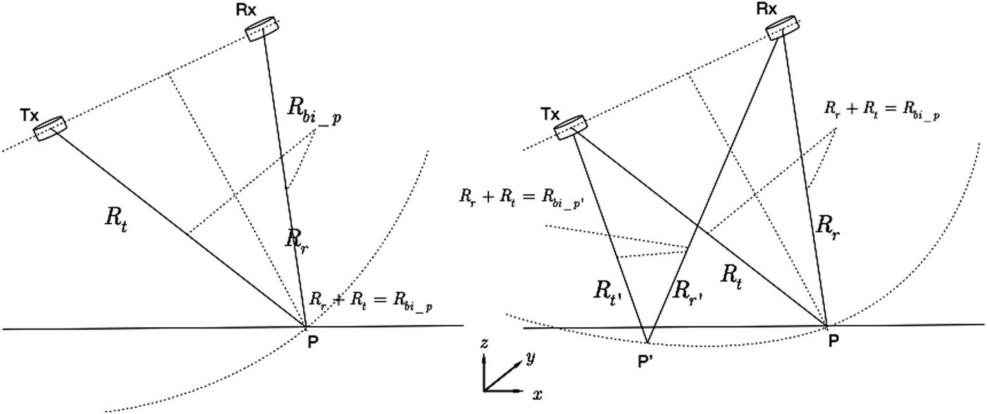
**FIGURE 8.28** The illustration of the spherical and ellipsoid surface of the backward bistatic and forward bistatic.

To further explore the properties of the bistatic range histories of the point $P' (x_{P',} y_{P'})$ and target point $P (x_{P,} y_{P})$ , the iso-bistatic range and iso-bistatic Doppler frequency during the entire synthetic aperture time are depicted in Figure 8.29. Note that for the backward bistatic mode (see Figure 8.29a), as both platforms move synchronously, all intersecting curves cross at one point, the target position. For the forward bistatic modes (see Figure 8.29b), the intersecting curves meet in two points P and P’, due to equal bistatic range histories. The two range histories, Doppler histories, are equal, creating dual but identical targets in the data domain, so that a “ghost target” may appear in the focused image. It is the difference of the projection rule that the difference between the backward and forward bistatic SAR.

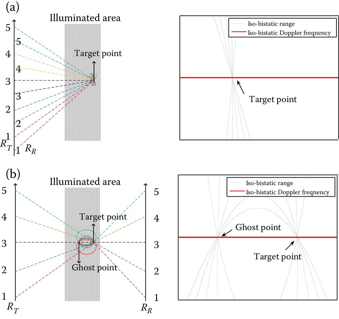
**FIGURE 8.29** The range histories of the backward bistatic (a) and forward bistatic (b) at target P during full aperture and the numbers 1–5 represent different positions of the transmitter and receiver at the azimuth direction. The right column is the zoom of the target imaging scene of the left column.

In the forward bistatic mode, we can locate the position of the ghost P’ of a certain target P with the conditions: for plane assumption, $Z_{R} = 0$ , and for ellipsoid, $R_{b i} (η_{i}) = R_{b i_P} (η_{i})$ ; where $R_{b i}$ is the bistatic range to the point in the imaging scene, $R_{b i_P}$ is the bistatic range to the target point and $η_{i}$ is the instantaneous azimuth time, slow time, during the target exposure period. In plane surface assumption, it means only the points on the earth plane are considered. The ellipsoid case means that the bistatic range of ghost image is equal to the bistatic range of target point in the whole observation time, which is often selected to increase the prediction accuracy of the position of ghost image.

8.5.4 EXAMPLES

For the purpose of simulation and to be more practical, we adopt the system parameters from SAOCOM-CS mission [46–48], as given in Table 8.4. In SAOCOM-CS mission, the bistatic incidence angle range is 20.7~38.4°. In our simulation, the incidence angle from the transmitter is selected as a central incidence angle 29.55°.

TABLE 8.4
Key Simulation Parameters for Bistatic Imaging

System/Motion	Parameter	Symbol	Value
System parameters	Chirp bandwidth	B	45 MHz
	Processed Doppler bandwidth	B_a	1050 Hz
	Center frequency	f_c	1275 MHZ
	Wavelength	λ	23 cm
	Integration time	T_a	10 s
	Transmitter peak power	P_T	3.1 kW
	Antenna gain of transmitter	$G_{T}$	55 dB
	Antenna gain of receiver	$G_{R}$	50 dB
	Receiver noise temperature	$T_{R}$	300 K
	Receiver noise figure	$F_{n}$	4.5 dB
	Propagation losses	$L$	3.5 dB
	Duty cycle	$D_{c}$	0.05
Motion parameters	Orbit height	$H$	619.6 km
	Transmitter incidence angle	$θ_{T}$	29.55°
	Transmitter azimuth angle	$φ_{T}$	0°
	Flight velocity	v	7545 m/s

In what follows, the imaging property of backward and forward bistatic SAR will be analyzed. This system works in the receiver incidence angle between 21° and 57° with 7 beams in total (3° on the left and right sides of the beam center) and its corresponding ground range resolution is shown in Figure 8.30.

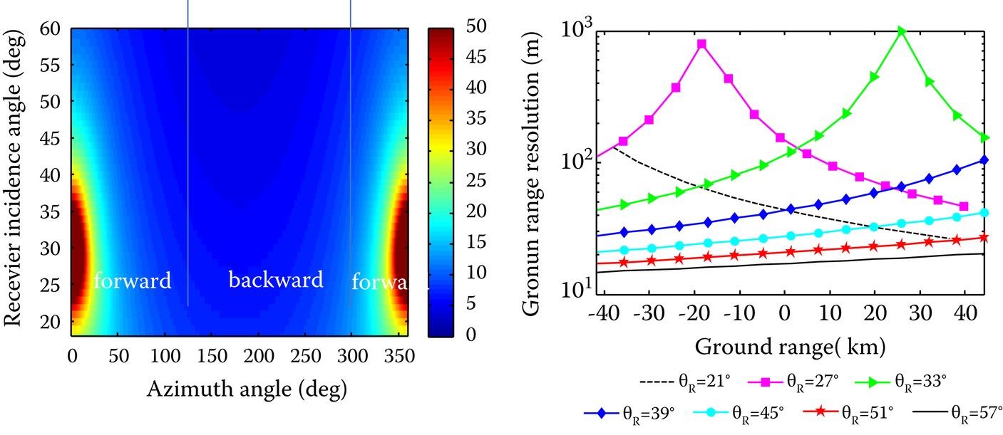
**FIGURE 8.30** (Left): The ground range resolution with respect to the received azimuth angle $φ_{R}$ . (Right): The ground range resolution in different beams.

We see that the ground range resolution in the backward mode is similar to monostatic SAR and that is beneficial for imaging. In addition, only in the forward scattering zone, the ground range resolution deteriorates and the phenomenon is more obvious as the incidence angle differences between the transmitter and the receiver become small, particularly near the specular region. In the forward specular bistatic, the transmitter and the receiver are symmetrical about the center region within the imaging scene. This symmetry causes the two opposite direction vectors in the x-axis to counteract each other and the resolution becomes extremely poor. As the angular difference between the transmitter and receiver becomes larger, the ground range resolution changes are mitigated and improve considerably. Thus, conclusions can be drawn that the ground range resolution in the backscattering zone is superior to that in the forward backscattering zone with a certain incidence angle. To improve the ground range resolution, the receiver incidence angle should be selected away from the transmitter incidence angle and the azimuth angle should be increased as much as possible. In addition, special attention should be paid to avoid the approximately symmetrical imaging configuration in the forward bistatic SAR.

Figure 8.31 shows the azimuth resolution with respect to the velocity direction angle β and azimuth angle $φ_{R}$ . It is seen that the azimuth resolution has a slight change when $β = 0^{°}$ , since the two SAR platforms move in the same direction with a parallel track. When the velocity angle is close to 180°, the azimuth resolution diverges, because the angular velocity vectors $w_{T} (η)$ and $w_{R} (η)$ are in opposition, which therefore is not recommended in bistatic SAR. The influence of the velocity direction angle is dominant and the receiver incidence angle adds to the effect. Conclusions that the opposite velocity vectors are not desirable even though the azimuth resolution becomes better as the receiver incidence angle changes. Except in the case of velocity angle near to 180°, there is not much difference for the azimuth resolution for backward and forward bistatic SAR.

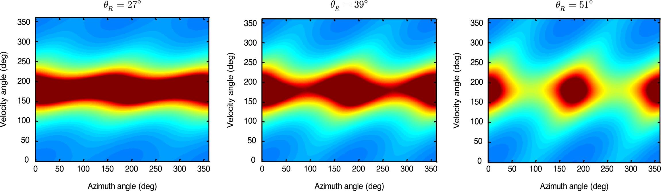
**FIGURE 8.31** The azimuth resolution with respect to velocity angle β and received azimuth angle $φ_{R}$ . with $θ_{T} = 29.55 °$ .

In most practical cases, the velocity angle is set zero, which means a parallel track. The ground range and azimuth resolutions, resolution direction angle, and the ground resolution cell area with respect to the azimuth angle and the receiver incidence angle, with $θ_{T} = {29.55}^{°}$ and $β = 0^{°}$ are plotted in Figure 8.32. Figure 8.32a shows that the azimuth resolution changes slightly in the whole scattering zone when $β = 0^{°}$ but it suffers degradation when $φ_{R}$ is near 90° and 270° because the sum of angular velocity units $w_{T} (η)$ and $w_{R} (η)$ is smaller. Figure 8.32b shows that the directions of the two resolutions are almost collinear in some regions in the forward scattering zone which causes defocus in the final image. Figure 8.32c also indicates the same trend; it can be seen that the areas with an orthogonal resolution direction angle are not strictly in conformity with the area with the smallest ground resolution cell and it is also influenced by the two ground resolutions. In some regions in the forward bistatic mode, the resolution cell is totally lost and should be avoided when designing the imaging geometric parameters.

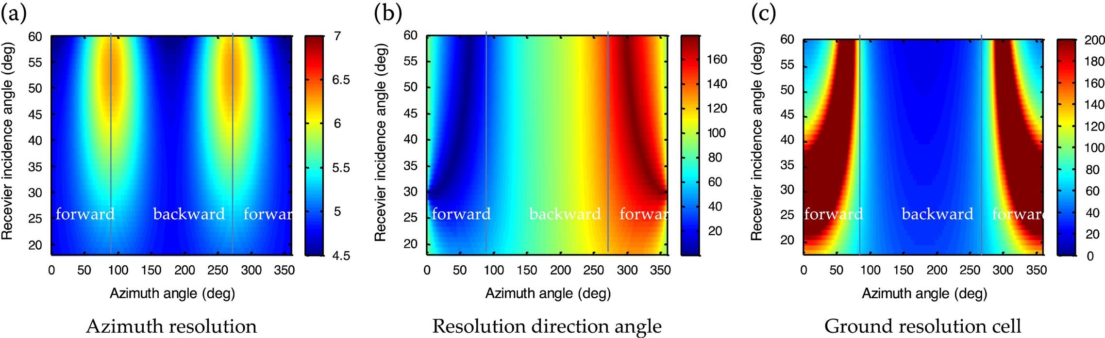
**FIGURE 8.32** The resolution analysis with respect to $θ_{R}$ . and $φ_{R}$ . . (a) Azimuth resolution; (b) Resolution direction angle; (c) Ground resolution cell with $θ_{T} = 29.55 °$ .

In the forward quasi-specular bistatic mode, the azimuth resolution is fine while the ground range resolution deteriorates rapidly, implying that the forward specular bistatic is not preferable for forward imaging in view of the resolution. In this simple demonstration, the geometric properties and power considerations of the backward and forward bistatic SAR are analyzed in a formation mode. In addition, the focus is on the forward bistatic configuration which has been proven to be beneficial for remote sensing applications. As predicted by the range history analysis and verified by the back-projection imaging simulation results, the bistatic range history phenomenon that introduces “ghost targets” exists when the imaging area is across the specular region. That drawback should be avoided by limiting the illumination area beside the specular region rather than across it. By enlarging the difference in the incidence angles of the transmitter ( $θ_{T}$ ) and receiver ( $θ_{R}$ ), the ghost-free area can be broadened for practical observations. From the view of realizing a sufficiently high resolution, the quasi-specular forward imaging geometry should also be avoided, as the ground range resolution deteriorates badly in this case. The azimuth resolution variation is relatively insignificant as long as the velocity directions of the transmitter and receiver are not notably different. Then, based on the considerations of the range ambiguity effect, the ground resolution cell area size, remarks on the forward bistatic SAR imaging geometry design can be concluded: a sufficiently large difference in the transmitting and receiving incidence angle ( $θ_{T}$ and $θ_{R}, θ_{R} > θ_{T}$ ) should be guaranteed near the incident plane, for ghost-free imaging and achieving a good balance between fine resolution and obtaining richer scattering features from earth surfaces.

Bistatic SAR is a fast-growing and active research area for its high potential of providing much richer information about the targets, including the geometric and dielectric properties. As we also demonstrated in Chapters 4 and 5, for remote sensing of soil moisture, bistatic scattering offers a much wider dynamic range and higher sensitivity in response to moisture content changes. The bistatic scattering measurement, if properly configured, also help to decouple the responses of surface roughness and moisture content, namely, the strong coupling between the geometric and dielectric properties can be better separated. More research efforts, however, should be devoted to better capture a more complete picture of the bistatic scattering pattern.

References

1. Ishimaru, A., Wave Propagation and Scattering in Random Media, Academic Press, New York, 1978.

2. Tsang, L., Kong, J. A., and Shin, R. T., Theory of Microwave Remote Sensing, Wiley, New York, 1985.

3. Fung, A. K., Microwave Scattering and Emission Models and Their Applications, Artech House, Norwood, MA, 1994.

4. Ulaby, F. T. and Long, D. G., Microwave Radar and Radiometric Remote Sensing, University of Michigan Press, Ann Arbor, MI, 2014.

5. Chew, W. C., Waves and Fields in Inhomogeneous Media, IEEE Press, Piscataway, NJ, 1995.

6. Chew, W. C., Jin, J. M., Michielssen, E., and Song, J., Fast and Efficient Algorithms in Computational Electromagnetics, Artech House, Norwood, MA, 2000.

7. Tsang, L., Kong, J. A., Ding, K. H., Scattering of Electromagnetic Waves: Theories and Applications, Wiley, New York, 2000.

8. Jing, J. M., Theory and Computation of Electromagnetic Fields, 2^nd edn Edition, Wiley-IEEE Press, New York, 2015.

9. Graglia, R. D., Peterson, A. F., Higher-Order Techniques in Computational Electromagnetics, SciTech Publishing, Raleigh, NC, 2016.

10. Tsang, L., Ding, K. H., Huang, S. W., and Xu, X. L., Electromagnetic computation in scattering of electromagnetic waves by random rough surface and dense media in microwave remote sensing of land surfaces, Proceedings of the IEEE, 101(2), 255–279, 2013.

11. Tsang, L., Liao, T.-H., Tan, S., Huang, H., Qiao, T., and Ding, K. H., Rough surface and volume scattering of soil surfaces, ocean surfaces, snow, and vegetation based on numerical Maxwell model of 3D simulations, IEEE Journal of Selected Topics in Applied Earth Observations and Remote Sensing, 10(11), 4703–4720, 2017.

12. Tsang, L., Cha, J. H., and Thomas, J. R., Electric Fields of spatial Green’s functions of microstrip structures and applications to the calculations of impedance matrix elements, Microwave and Optical Technology Letters, 20(2), 90–97, 1999.

13. Li., Q., Chan, H., and Tsang, L., Monte-Carlo simulations of wave scattering from lossy dielectric random rough surfaces using the physics-based two-gird method and canonical grid method, IEEE Transactions on Antennas and Propagation, 47(4), 752–763, 1999.

14. Arfken, G., Mathematical Methods for Physicists, 3^rd edn Edition, Academic Press, Orlando, FL, 1985.

15. Chen, X. D., Computational Methods for Electromagnetic Inverse Scattering, Wiley-IEEE Press, Hoboken, NJ, 2018.

16. Keller, J. B., Accuracy and validity of the Born and Rytov pproximations. Journal of the Optical Society of America, 59(8), 1003, 1969.

17. Marks, D. L., A family of approximations spanning the Born and Rytov scattering series, Optics Express, 14(19), 8837, 2006.

18. Levy, M., Parabolic Equation Mescattering media on super thods for Electromagnetic Wave Propagation. IET, London, 2000.

19. Zhang, P., Bai, L., Wu, Z., and Guo, L., Applying the parabolic equation to tropospheric groundwave propagation: A review of recent achievements and significant milestones, IEEE Antennas and Propagation Magazine, 58(3), 31–44, 2016.

20. Devaney, A. J., Time reversal imaging of obscured targets from multistatic data, IEEE Transactions on Antennas and Propagation, 53(5), 1600–1610, 2005.

21. Devaney, A. J., Mathematical Foundations of Imaging, Tomography and Wavefield Inversion, Cambridge University Press, Cambridge, UK, 2012.

22. Ishimura, A., Electromagnetic Wave Propagation, Radiation, and Scattering: From Fundamentals to Applications, 2^nd edn Edition, Wiley-IEEE Press, Hoboken, NJ, 2017.

23. Ishimaru, A., Jaruwatanadilok, S., & Kuga, Y., Time reversal effects in random scattering media on super-resolution, shower curtain effects, and backscattering enhancement. Radio Science, 42(6), RS6S28. 2007. doi:10.1029/2007RS003645

24. Ishimaru, A., Jaruwatanadilok, S., and Kuga, Y., Imaging through random multiple scattering media using integration of propagation and array signal processing, Waves in Random & Complex Media, 22(1): 24–39, 2012.

25. Goodman, J. W., 2^nd edn Edition, Statistical Optics, Wiley, New York, 2015.

26. Chan, T., Jaruwatanadilok, S., Kuga, Y., and Ishimura, A., Numerical study of the time-reversal effects on super-resolution in random scattering media and comparison with an analytical model, Waves in Random & Complex Media, 18(4), 627–639, 2008.

27. Cumming, I., and Wong, F., Digital Signal Processing of Synthetic Aperture Radar Data: Algorithms and Implementation, Artech House, Norwood, MA, 2004.

28. Chiang C. Y., Chen K. S. Simulation of complex target RCS with application to SAR image recognition 3rd International Asia-Pacific Conference on Synthetic Aperture Radar (APSAR), Seoul, Korea, 1-4, 26–30 September 2011

29. Chen, K. S., Principles of Synthetic Aperture Radar: A System Simulation Approach . CRC Press: Boca Raton, FL, 2015.

30. Ku, C. S., Chen, K. S., Chang, P. C., and Chang, Y. L., Imaging simulation of synthetic aperture radar based on full wave method, Remote Sensing, 10(9), 1404, 2018.

31. Piepmeier, J. R., and Simon, N. K., A polarimetric extension of the van Cittert-Zernike Theorem for use with microwave interferometers, IEEE Geoscience and Remote Sensing Letters, 1(4), 300–303, 2004.

32. Born, M., and Wolf, E., Principles of Optics, 7^th edn Edition, Cambridge University Press, New York, 1999.

33. Hong, S. T., and Ishimaru, A., Two-frequency mutual coherence function, coherence bandwidth, and coherence time of millimeter and optical waves in rain, fog, and turbulence. Radio Science, 11, 551–559, 1976.

34. Ishimaru, A., Ailes-Sengers, L., Phu, P., and Winebrenner, D., Pulse broadening and two-frequency mutual coherence function of the scattered wave from rough surfaces, Waves Random Media, 4, 139–148, 1994.

35. Kuga, Y., Le, T. C. C., Ishimaru, A., and Ailes-Sengers, L., Analytical, experimental, and numerical studies of angular memory signatures of waves scattered from one-dimensional rough surfaces, IEEE Transactions on Geoscience and Remote Sensing, 34(6), 1300–1307, 1996.

36. Tsang, L., Zhang, G., and Pak, K., Detection of a buried object under a single random rough surface with angular correlation function in EM wave scattering, Microwave and Optical Technology Letters, 11(6), 300–304, 1996.

37. Zhang, G., Tsang, L., and Kuga, Y., Studies of the angular correlation function of scattering by random rough surfaces with and without a buried object, IEEE Transactions on Geoscience and Remote Sensing, 35(2), 444–453, 1997.

38. Guo, L. X., Wu, Z. S., Study on the two-frequency scattering cross section and pulse broadening of the one-dimensional fractal sea surface at millimeter wave frequency. Progress in Electromagnetic Research, 37, 221–234, 2002.

39. Wu, K., Two-frequency mutual coherence function for electromagnetic pulse propagation over rough surfaces, Waves in Random and Complex Media, 15(2), 127–143, 2005.

40. Ren, Y., Guo, L., Two-frequency mutual coherence function and its applications to pulse scattering by random rough surface, Science China Physics, Mechanics, & Astronomy, 51, 157–164, 2008.

41. Le, C. T., Kuga, Y., and Ishimaru, A., Angular correlation function based on the second-order Kirchhoff approximation and comparison with experiments, Journal of Optical Society of America A, 13(5), 1057–1067, 1996.

42. Li, T., Chen, K. S., and Jin, M., Analysis and simulation on imaging performance of backward and forward bistatic SAR, Remote Sensing, 10, 1676, 2018.

43. Cardillo, G. P., On the use of the gradient to determine bistatic SAR resolution, Proceedings of Antennas and Propagation Society International Symposium, Dallas, TX, USA, 7–11 May; 1032–1035, 1990 10.1109/APS.1990.115286.

44. Moccia, A., and Renga, A., Spatial resolution of bistatic synthetic aperture radar: Impact of acquisition geometry on imaging performance, IEEE Transactions on Geoscience and Remote Sensing, 49(10), 3487–3503, 2011.

45. Qiu, X. L., Ding, C. B., Hu, D. H., Bistatic SAR Data Processing Algorithms, John Wiley Sons, New York, 2013.

46. Gebert, N., Dominguez, B. C., Davidson, M. W. J., Martin, M. D., and Silvestrin, P., SAOCOM-CS—apA passive companion to SAOCOM for single-pass L-band SAR interferometry. In Proceedings of 2014 10th European Conference on Synthetic Aperture Radar, Berlin, Germany, 1–4, 3–5 June 2014.

47. Bordoni, F., Younis, M., Cassola, M. R., Iraol, P. P., Dekker, P. L., Krieger, G. SAOCOM-CS SAR imaging performance evaluation in large baseline bistatic configuration. Proceedings of 2015 IEEE International Geoscience and Remote Sensing Symposium, Milan, Italy, 26–31 July 2015; 2107–2110, 10.1109/IGARSS.2015.7326218.

48. Gebert, N., Dominguez, B. C., Martin, M. D., Salvo, E. D., Temussi, F., Giove, P.V., Gibbons, M., Phelps, P., and Griffiths, L., SAR Instrument Pre-development Activities for SAOCOM-CS. Proceedings of 2016 11th European Conference on Synthetic Aperture Radar (EUSAR), Hamburg, Germany, 1–4, 6–9 June 2016.

APPENDIX 8A

Explicit forms of ${\vec{I}}^{r}$ and ${\vec{F}}^{r}$

For simple notation, let

${\bar{\bar{G}}}_{t}^{d} \equiv [\begin{matrix} \hat{x} \hat{x} G_{x x} & \hat{x} \hat{y} G_{x y} & \hat{x} \hat{x} G_{x z} \\ \hat{y} \hat{x} G_{y x} & \hat{y} \hat{y} G_{y y} & \hat{y} \hat{z} G_{y z} \\ \hat{z} \hat{x} G_{z x} & \hat{z} \hat{y} G_{z y} & \hat{z} \hat{z} G_{z z} \end{matrix}]$ (8.A1)

$\nabla \times {\bar{\bar{G}}}_{t}^{d} = [\begin{matrix} \hat{x} \hat{x} D_{x x} & \hat{x} \hat{y} D_{x y} & \hat{x} \hat{x} D_{x z} \\ \hat{y} \hat{x} D_{y x} & \hat{y} \hat{y} D_{y y} & \hat{y} \hat{z} D_{y z} \\ \hat{z} \hat{x} D_{z x} & \hat{z} \hat{y} D_{z y} & \hat{z} \hat{z} D_{z z} \end{matrix}]$ (8.A2)

After a series of vector manipulations, we can obtain

$I_{x}^{r} = \hat{x} \cdot {\overset{⇀}{I}}^{r} = \hat{x} \cdot (\vec{s} \times {\overset{⇀}{E}}^{i}) + \hat{x} \cdot \vec{s} \times \iint (\nabla \times \bar{\bar{G}} \cdot {\overset{⇀}{I}}^{r'} + j ω μ \bar{\bar{G}} \cdot {\overset{⇀}{F}}^{r'}) d x' d y' = - E_{i y} + \iint {[(- ξ_{y} D_{z x} - D_{y x}) + ξ_{x}^{'} (- ξ_{y} D_{z z} - D_{y z})] I_{x}^{r'} + [(- ξ_{y} D_{z y} - D_{y y}) + ξ_{y}^{'} (- ξ_{y} D_{z z} - D_{y z})] I_{y}^{r'} + j ω μ [(- ξ_{y} G_{z x} - G_{y x}) + ξ_{x}^{'} (- ξ_{y} G_{z z} - G_{y z})] F_{x}^{r'} + j ω μ [(- ξ_{y} G_{z y} - G_{y y}) + ξ_{y}^{‘} (- ξ_{y} G_{z z} - G_{y z})] F_{y}^{r'}} d x' d y'$ (8.A3)

$I_{y}^{r} = \hat{y} \cdot {\overset{⇀}{I}}^{r} = \hat{y} \cdot (\vec{s} \times {\overset{⇀}{E}}^{i}) + \hat{y} \cdot \vec{s} \times \iint (\nabla \times \bar{\bar{G}} \cdot {\overset{⇀}{I}}^{r'} + j ω μ \bar{\bar{G}} \cdot {\overset{⇀}{F}}^{r'}) d x' d y' = E_{i x} + ξ_{x} E_{i y} + \iint {[(D_{x x} + ξ_{x} D_{z x}) + ξ_{x}^{'} (D_{x z} + ξ_{x} D_{z z})] I_{x}^{r'} + [(D_{x y} + ξ_{x} D_{z y}) + ξ_{y}^{'} (D_{x z} + ξ_{x} D_{z z})] I_{y}^{r'} + j ω μ [(G_{x x} + ξ_{x} G_{z x}) + ξ_{x}^{‘} (G_{x z} + ξ_{x} G_{z z})] F_{x}^{r'} + j ω μ [(G_{x y} + ξ_{x} G_{z y}) + ξ_{y}^{'} (G_{x z} + ξ_{x} G_{z z})] F_{y}^{r'}} d x' d y'$ (8.A4)

$F_{x}^{r} = \hat{x} \cdot {\overset{⇀}{F}}^{r} = \hat{x} \cdot (\vec{s} \times {\overset{⇀}{H}}^{i}) + \hat{x} \cdot \vec{s} \times \iint {- j ω ε (\bar{\bar{G}} \cdot {\overset{⇀}{I}}^{r'}) + (\nabla \times \bar{\bar{G}} \cdot {\overset{⇀}{F}}^{r'})} d x' d y' = - H_{i z} - β H_{i y} + \iint {- j ω ε [(- ξ_{y} G_{z x} - G_{y x}) + ξ_{x}^{'} (- ξ_{y} G_{z z} - G_{y z})] I_{x}^{r'} - j ω ε [(- ξ_{y} G_{z y} - G_{y y}) + ξ_{y}^{'} (- ξ_{y} G_{z z} - G_{y z})] I_{y}^{r'} + [(- ξ_{y} D_{z x} - D_{y x}) + ξ_{x}^{'} (- f_{y} D_{z z} - D_{y z})] F_{x}^{r'} + [(- ξ_{y} D_{z y} - D_{y y}) + ξ_{y}^{'} (- ξ_{y} D_{z z} - D_{y z})] F_{y}^{r'} d x' d y'$ (8.A5)

$\begin{array}{l} F_{y}^{r} & = & \hat{y} \cdot {\overset{⇀}{F}}^{r} \\ = & \hat{y} \cdot (\vec{s} \times {\overset{⇀}{H}}^{i}) + \hat{y} \cdot \vec{s} \times \iint {- j ω ε (\bar{\bar{G}} \cdot {\overset{⇀}{I}}^{r'}) + (\nabla \times \bar{\bar{G}} \cdot {\overset{⇀}{F}}^{r'})} d x' d y' \\ = & - H_{i y} - ξ_{y} H_{i y} + \iint {- j ω ε [(G_{x x} + f_{x} G_{z x}) + ξ_{x}^{'} (G_{x y} + ξ_{x} G_{z y})] I_{x}^{r'} \\ - j ω ε [(G_{x y} + ξ_{x} G_{z y}) + ξ_{y}^{'} (G_{x z} + ξ_{x} G_{z z})] I_{y}^{r'} + \\ [(D_{x x} + ξ_{x} D_{z x}) + ξ_{x}^{'} (D_{x y} + ξ_{x} D_{z y})] F_{x}^{r'} + [(D_{x y} + ξ_{x} D_{z y}) + ξ_{y}^{'} (D_{x z} + ξ_{x} D_{z z})] F_{y}^{r'} d x' d y \end{array}$ (8.A6)

Note that

$\hat{n} \cdot {\overset{⇀}{I}}^{r} = 0 \to I_{z}^{r} = ξ_{x} I_{x}^{r} + ξ_{y} I_{y}^{r}$ (8.A7)

$\hat{n} \cdot {\overset{⇀}{F}}^{r} = 0 \to F_{z}^{r} = ξ_{x} F_{x}^{r} + ξ_{y} F_{y}^{r}$ (8.A8)

It follows that the normal components of ${\vec{I}}^{r}$ and ${\vec{F}}^{r}$ are written as, respectively

$I_{n}^{r} = (- ξ_{x} E_{i x} - ξ_{y} E_{i y} + E_{i z}) + \int {[- (ξ_{x} D_{x x} + ξ_{y} D_{y x} - D_{z x} + ξ_{x} ξ_{x}^{'} D_{x z} + ξ_{y} ξ_{x}^{'} D_{y z} - ξ_{x}^{'} D_{z z}] I_{x}^{r'} + [ξ_{x} D_{x y} + ξ_{y} D_{y y} - D_{z y} + ξ_{x} ξ_{x}^{'} D_{x z} + ξ_{y} ξ_{x}^{'} D_{y z} - ξ_{x}^{'} D_{z z}] I_{y}^{r'} - j ω ε [ξ_{x} G_{x x} + ξ_{y} G_{y x} - G_{z x} + ξ_{x} ξ_{x}^{'} G_{x z} + ξ_{y} ξ_{x}^{'} G_{y z} - ξ_{x}^{'} G_{z z}] F_{x}^{r'} + j ω ε [ξ_{x} G_{x y} + ξ_{y} G_{y y} - G_{z y} + ξ_{x} ξ_{y}^{'} G_{x z} + ξ_{y} ξ_{y}^{'} G_{y z} - ξ_{y}^{'} G_{z z}] F_{y}^{r'}} d x' d y'$ (8.A9)

$F_{n}^{r} = (- ξ_{x} H_{i x} - ξ_{y} H_{i y} + H_{i z}) + \iint {(- i ω ε) [ξ_{x} G_{x x} + ξ_{y} G_{y x} - G_{z x} + ξ_{x} ξ_{x}^{'} G_{x z} + ξ_{y} ξ_{x}^{'} G_{y z} - ξ_{x}^{'} G_{z z}] I_{x}^{r'} + (- j ω ε) [ξ_{x} G_{x y} + ξ_{y} G_{y y} - G_{z y} + ξ_{x} ξ_{y}^{'} G_{x z} + ξ_{y} ξ_{y}^{'} G_{y z} - ξ_{y}^{'} G_{z z}] I_{y}^{r'} - [ξ_{x} D_{x x} + ξ_{y} D_{y x} - D_{z x} + ξ_{x} ξ_{x}^{'} D_{x z} + ξ_{y} ξ_{x}^{'} D_{y z} - ξ_{x}^{'} D_{z z}] F_{x}^{r'} + [ξ_{x} D_{x y} + ξ_{y} D_{y y} - D_{z y} + ξ_{x} ξ_{y}^{'} D_{x z} + ξ_{y} ξ_{y}^{'} D_{y z} - ξ_{y}^{'} D_{z z}] F_{y}^{r'}} d x' d y'$ (8.A10)

APPENDIX 8B

Explicit forms of ${\bar{\bar{G}}}_{t}^{r}$ and $\nabla \times {\bar{\bar{G}}}_{t}^{r}$

To write explicit forms of ${\bar{\bar{G}}}_{t}^{r}$ and $\nabla \times {\bar{\bar{G}}}_{t}^{r}$ , let $X = x - x', Y = y - y', Z = z + z' + 2 d_{1}$ , with $Δ = e^{- i 2 k_{t z} d_{1}}$ , and $ρ = \sqrt{X^{2} + Y^{2}}$ , $φ = \tan^{- 1} (Y / X)$ . After some mathematical manipulations, we have

In Equations 8.B1 and 8.B2, J_n is Bessel function of order n and ${J'}_{n}$ is derivative of Bessel function of order n. It is noted that the $\hat{z} \hat{z}$ component vanishes.

Tags: Radar Scattering and Imaging of Rough Surfaces Modeling and Applications with MATLAB

Jul 18, 2021 | Posted by admin in General Engineer | Comments Off

Engineer Key

Fastest Engineer Engine

Radar Imaging Techniques