7 Selected Model Applications to Remote Sensing
An analytical scattering model presented in Chapter 4 has been validated by comparison with numerical simulations and measurements from ground-based, airborne, and spaceborne sensors. The sensitivity test on the surface parameters response to radar return was presented in Chapter 5. In the previous chapter, issues regarding the parameter estimation from radar measurements have been discussed. The mapping from parameter domain to data (or image) domain, and vice versa, is a highly nonlinear problem. Various techniques for information retrieval from remotely sensed data have been proposed in many recent studies—they are too numerous to cite all of them here. Some of them are based on an empirical relationship between the measured return signals and the ground truth. Because they developed from a limited number of observations, these models are generally valid only for the conditions under which those measured data were taken. For example, some of these models also appear that no dependence on the roughness parameter, correlation length. In this chapter, we presented a few model application examples: soil moisture retrieval and directional finding of the incident source.
If one perceives radar remote sensing—a stochastic electromagnetic wave scattering problem—more closely and deeply, the following the 4Vs characteristics may be recognized: volume, variety, velocity, and veracity. As pointed out by Hey et al. [1], the data science in the big data era combines and synergizes the observation, model prediction, and numerical simulation such that data transforms into information, and knowledge can be assured. Within a context of radar imaging, as we see from the 4Vs, more advanced data analytics apparently should be developed to explore richer information offered by fully bistatic radars with fully polarized remote sensing data, which is the main objective of this paper. Hence, it can be realized that a better solution of inverting rough surface parameters is that, by knowing the scattering patterns, one may be able to detect the presence of undesired random roughness of a reflective surface (e.g., an antenna reflector), and thus accordingly, and perhaps effectively, devise a means to correct or compensate phase errors. In many aspects, parameters retrieval from radar measurements is a highly nonlinear problem, yet an important objective in radar remote sensing of surfaces. The advance of neural network and deep learning [2–4] has provided an effective and yet efficient approach to retrieving these surface parameters.
7.1 SURFACE PARAMETER RESPONSE TO RADAR OBSERVATIONS—A QUICK LOOK
To get started, we present the AIEM backscattering predictions with experimental measurements from ground-based, airborne, and spaceborne sensors. Sample data from POLARSCAT Data [5], EMSL data [6], and SMOSREX06 Data [7] are used to illustrate the radar response to the surface parameters, though more details have been presented in previous chapters. These data were summarized and discussed in [8].
7.1.1 COMPARISON WITH POLARSCAT DATA
Remember that in Chapter 4, we illustrated a model prediction comparing with these data sets, but in a manner of correlation plot. The correlation plots of backscattering coefficients between the AIEM and the measured data for HH, VV, and HV polarizations are shown in Figures 4.12 and 4.13. Figure 4.12 shows the data for three frequency bands, and Figure 4.13 shows the data by separating the wet and dry conditions. Here, we would like to expand the comparison into more detail [8].
7.1.1.1 For Surface 1 (S1)
A total of three different soil surfaces with exponential autocorrelation function measured at three different frequencies (1.5, 4.75, and 9.5 GHz) ranging from 20° to 50° were used. The comparisons of AIEM predictions with the POLARSCAT measurements under different soil surfaces. The backscattering coefficients simulated by AIEM for an exponentially correlated surface with σ = 0.4 cm, = 8.4 cm at L/C/X-band under dry and wet soil conditions, are shown in Figures 7.1 and 7.2, respectively. It is seen visually that the angular trends of AIEM predictions generally coincide with the POLARSCAT data at all three frequencies. As expected, the backscattering coefficient decreases with increasing incident angle and increases with decreasing frequency from a smooth surface. Besides, it can be observed that the AIEM predictions agree better with the POLARSCAT data at smaller incident angles (e.g., 20° and 30°) while slightly deviate at lager incident angle (e.g., 40° and 50°), especially for HH polarization.
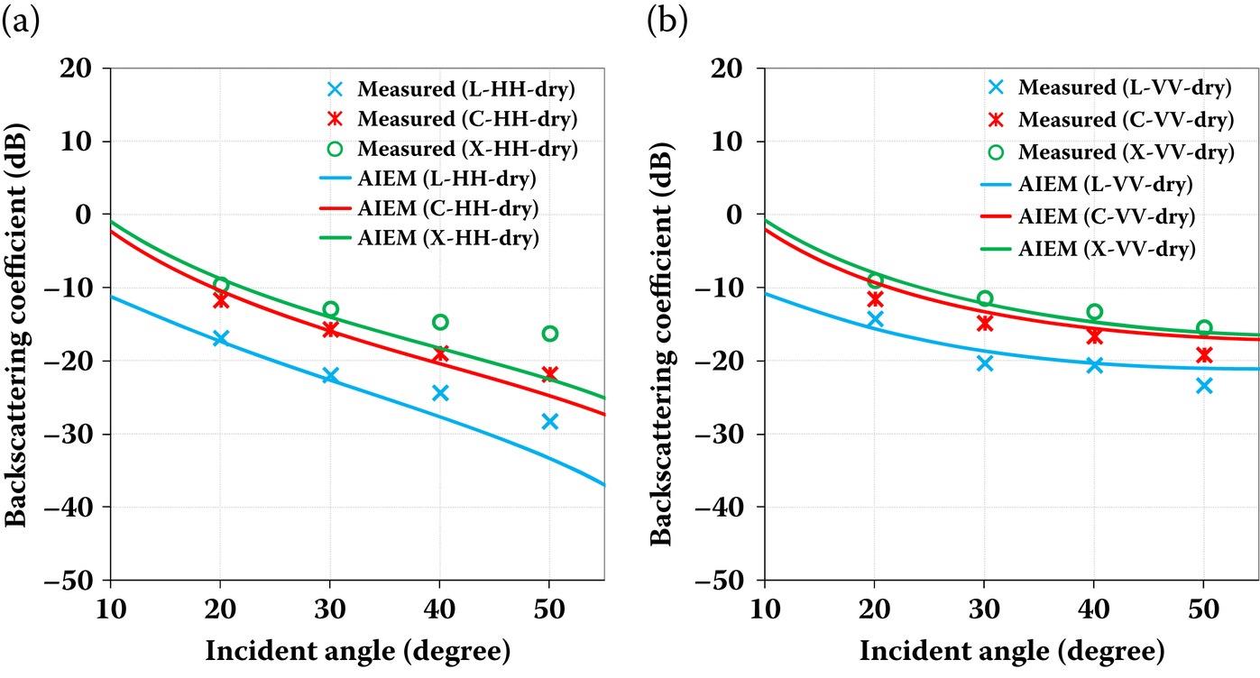
FIGURE 7.1 Comparison of backscattering coefficient between AIEM and POLARSCAT data for an exponential correlated surface with σ = 0.4 cm, = 8.4 cm at 1.5 GHz ( = 7.99-j2.02), 4.75 GHz ( = 8.77-j1.04) and 9.5 GHz ( = 5.70-j1.32) for (a) HH polarization and (b) VV polarization.
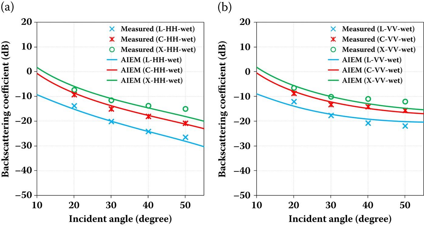
FIGURE 7.2 Comparison of backscattering coefficient between AIEM and POLARSCAT data for an exponential correlated surface with σ = 0.4 cm, = 8.4 cm at 1.5 GHz ( = 15.57-j3.71), 4.75 GHz ( = 15.42-j2.15) and 9.5 GHz ( = 12.31-j3.55) for (a) HH polarization and (b) VV polarization.
7.1.1.2 For Surface 2 (S2)
We compare the model predictions with the measurement data for the second soil surface (i.e., S2), and the results are shown in Figures 7.3 and 7.4. In general, the AIEM predictions are in good agreement with the POLARSCAT measurements over the most of the angular range under consideration, but deviates for HH polarization for incident angle larger than 40° under the dry soil conditions. It can be observed that the experimental measurements do not decrease monotonically with the increase of incident angle particularly for the L-band under dry soil conditions. This perhaps was attributed from measurement noises. As observed from the results of surface 1, the AIEM performs much better under wet soil conditions than under dry conditions for surface 2. This may be explained by the gradually increase of volume scattering in the dry soil surfaces that is somehow difficult to characterize [9].
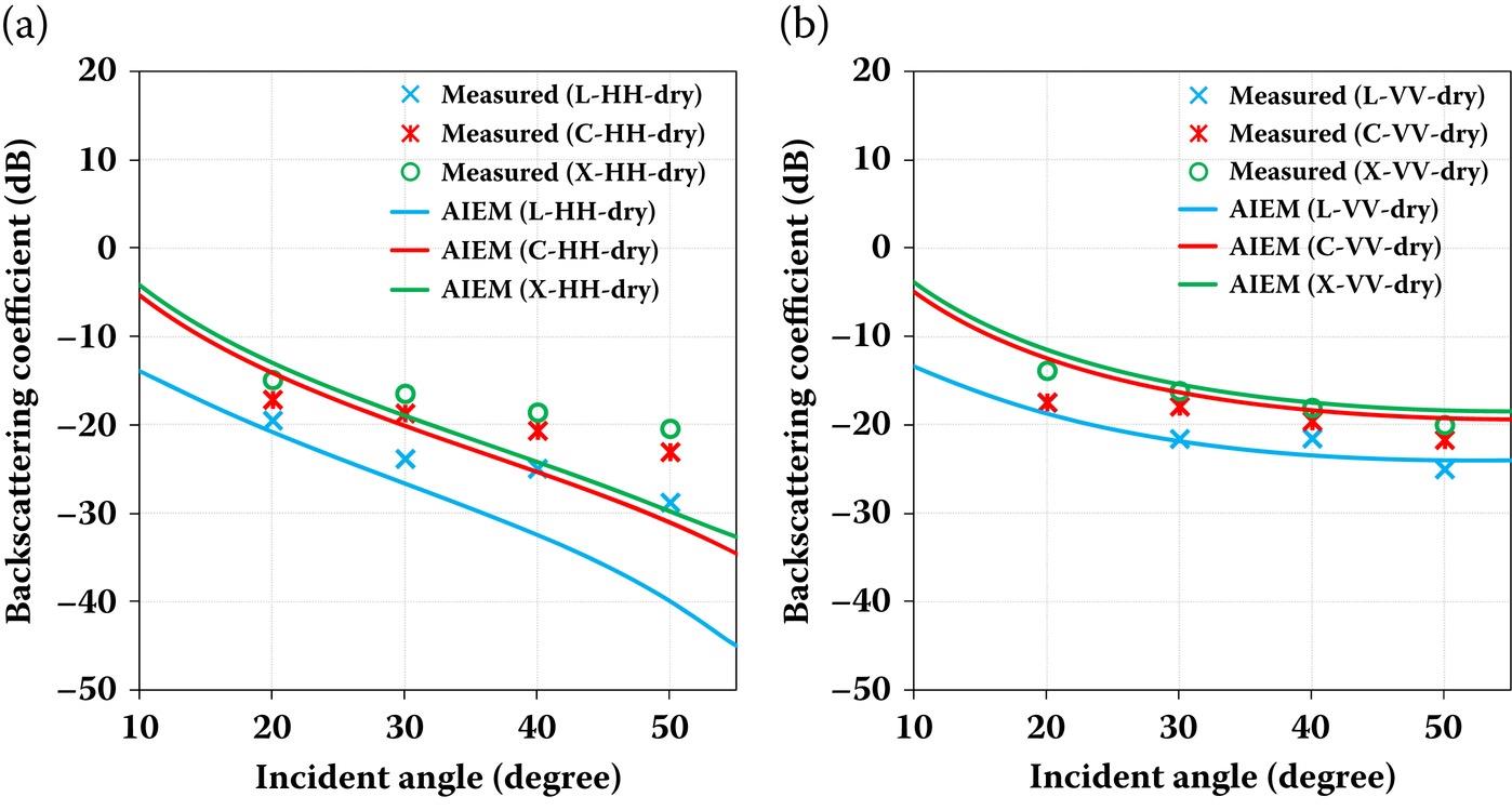
FIGURE 7.3 Comparison of backscattering coefficient between AIEM and POLARSCAT data for an exponential correlated surface with σ = 0.32 cm, = 9.9 cm at 1.5 GHz ( = 5.85-j1.46), 4.75 GHz ( = 6.66-j0.68) and 9.5 GHz ( = 4.26-j0.76) for (a) HH polarization and (b) VV polarization.
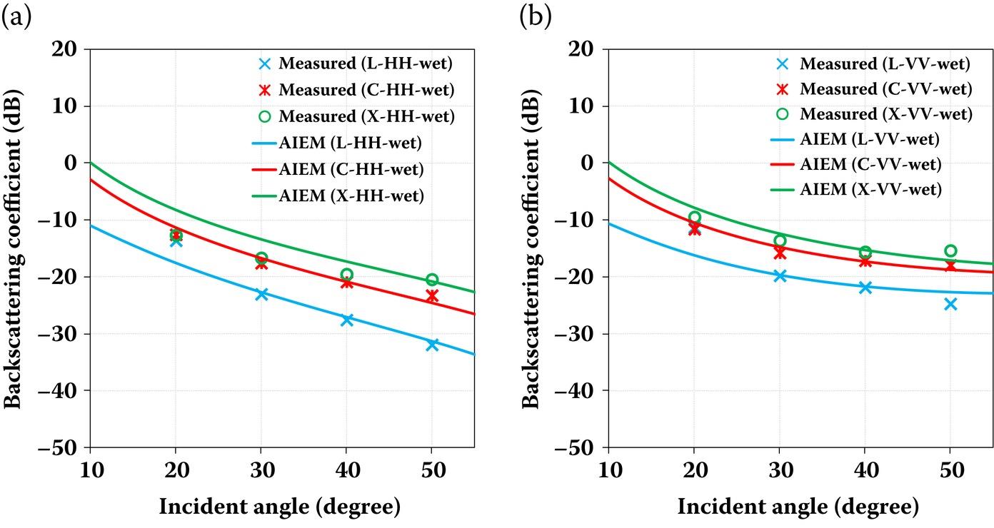
FIGURE 7.4 Comparison of backscattering coefficient between AIEM and POLARSCAT data for an exponential correlated surface with σ = 0.32 cm, = 9.9 cm at 1.5 GHz ( = 14.43-j3.47), 4.75 GHz ( = 14.47-j1.99) and 9.5 GHz ( = 12.64-j3.69) for (a) HH polarization and (b) VV polarization.
7.1.1.3 For Surface 3 (S3)
In what follows, we continue to assess the accuracy of AIEM backscattering simulations with the POLARSCAT data, shown in Figures 7.5 and 7.6. In this case, the RMS height is 1.12 cm, and the correlation length is 8.4 cm, which corresponds to the roughest surface among the three experiments. Due to the increased roughness, the scattering curve over all angles becomes flat. Again, the AIEM predictions well capture the angular trends of the POLARSCAT data at all frequencies for both HH and VV polarizations. It is also observed that in this case, the measurements at C-band and X-band are nearly the same regardless of the incident angle, whereas there is an obvious separation between the HH and VV polarized backscattering coefficient predicted by the AIEM over the incident angles. Insofar, we only illustrate the co-polarization. For discussion on cross-polarized backscattering, please refer to Chapter 4, and reference [10] for details.
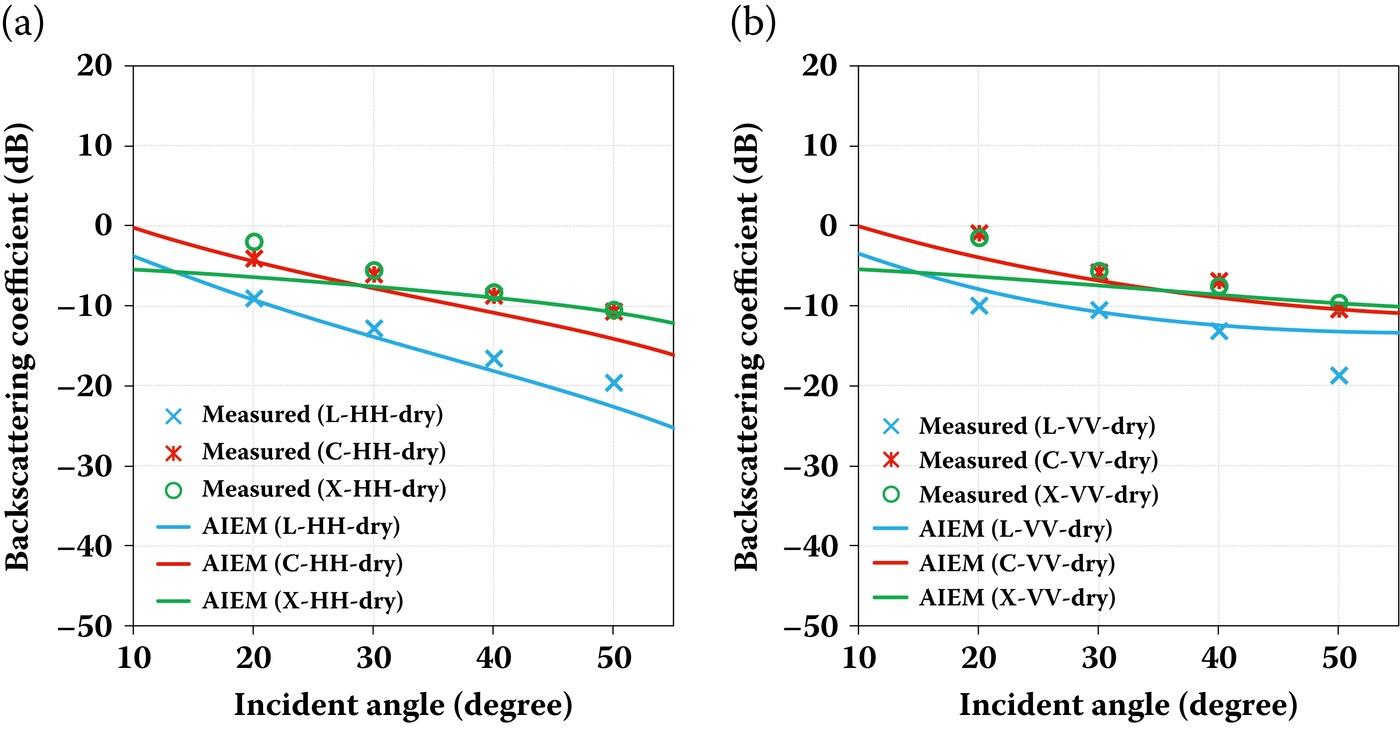
FIGURE 7.5 Comparison of backscattering coefficient between AIEM and POLARSCAT data for an exponential correlated surface with σ = 1.12 cm, = 8.4 cm at 1.5 GHz ( = 7.70-j1.95), 4.75 GHz ( = 8.50-j1.00) and 9.5 GHz ( = 6.07-j1.46) for (a) HH polarization and (b) VV polarization.
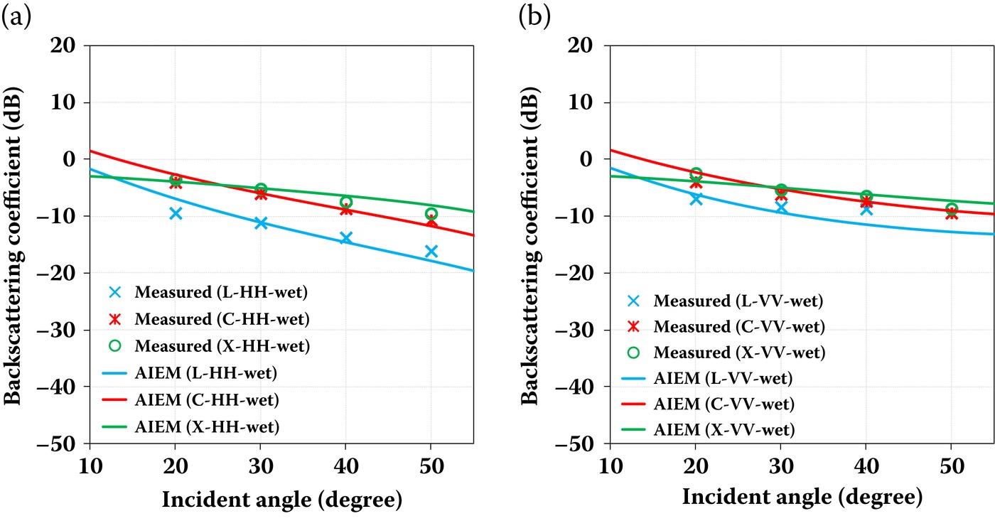
FIGURE 7.6 Comparison of backscattering coefficient between AIEM and POLARSCAT data for an exponential correlated surface with σ = 1.12 cm, = 8.4 cm at 1.5 GHz ( = 15.34-j3.66), 4.75 GHz ( = 15.23-j2.12) and 9.5 GHz ( = 13.14-j3.85) for (a) HH polarization and (b) VV polarization.
7.1.2 COMPARISON WITH EMSL DATA
The bistatic scattering measurement data used here was acquired by the EMSL [6]. The EMSL data were performed on a Gaussian correlated surface with σ = 0.4 cm, = 6 cm, and incident angle of 20° and scattering angle between 0° and 50° at two frequencies (i.e., 11 and 13 GHz). The comparison between the AIEM predictions and the EMSL measurements is shown in Figure 7.7. It can be observed that the bistatic scattering behavior of AIEM is generally in agreement with the EMSL data. The flatness of the angular trend between (10° and 30°), a forward scattering region, in measurements seems unexplainable, because in these scattering angles, a stronger scattering signal is physically expected. Nevertheless, the AIEM well predicts the bistatic scattering measurements for both HH and VV polarizations with a favorable RMSE value within 2.5 dB and a correlation value greater than 0.96.
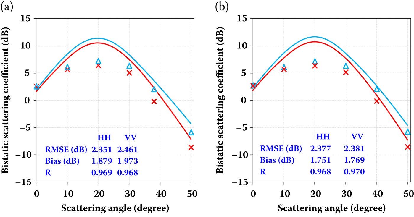
FIGURE 7.7 Comparison of bistatic scattering coefficient between AIEM and EMSL measurements for a Gaussian correlated surface with = 5.5-j2.1, σ = 0.4 cm, = 6 cm, and incident angle of 20° for (a) 11 GHz and (b) 13 GHz.
7.1.3 COMPARISON WITH SMOSREX06 DATA
For a rough surface, the noncoherent reflectivity is obtained by integrating the bistatic scattering coefficient over the upper hemisphere. Because of the reciprocity, the emissivity is the same as absorptivity, the amount of power absorbed by the dielectric in a scattering problem. Hence, it would be useful to examine the model prediction of the surface emissivity. Also, in this regard, the active and passive microwave remote sensing is interplayed.
The comparisons of the emissivity predicted by AIEM and the SMOSREX06 measurements are illustrated in Figure 7.8. Here, the performances of AIEM are observed in terms of angular and polarization dependences. It is seen that, in general, the AIEM predictions are fairly close to the measured emissivity at small to intermediate look angles, from 20° to 40°, for both H and V polarizations. However, when the look angle increases to 50° and 60°, the gap between these two data becomes larger, especially for H polarization. It is found that both the H and V polarized emissivities simulated by AIEM underestimate the SMOSREX06 measurements. Increasing the look angle, the dry bias at H polarization also increases, which is not observed at V polarization, however. Indeed, the RMSE is not quite satisfactory, particularly at large look angles (e.g., 50° and 60°) for H polarization. The AIEM predictions correlate well with the measured emissivity with the correlation coefficient close to 0.9 for both H and V polarizations. In Figure 7.8, we see a fairly well linear relationship between the AIEM predictions and measurements. Since the observation period of the measurements is very long, collecting a total of 8125 samples and the comparison, as presented here, is made without adjusting the given input parameters to the AIEM model, it is convinced that the AIEM is able to correctly predict the temporal dynamic of the observed surface emissivity over a wide range of look angle and surface parameters. More on the error measures are referred to [8].
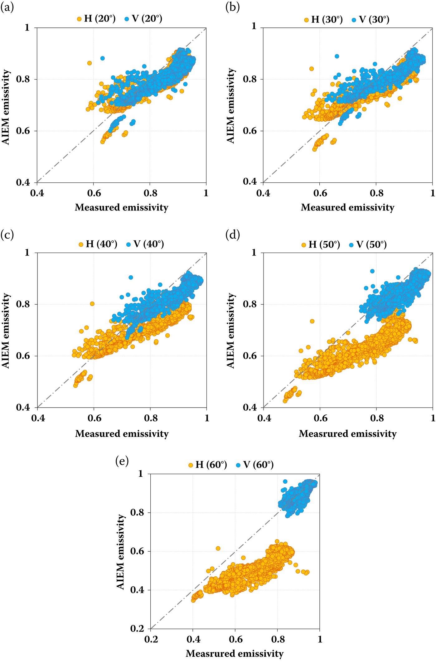
FIGURE 7.8 Comparison of H and V polarized emissivity between AIEM and SMOSREX06 measurements for an exponential correlated surface at 1.41 GHz with look angle of (a) 20°, (b) 30°, (c) 40°, (d) 50°, and (f) 60°.
7.2 SURFACE PARAMETER RETRIEVAL
7.2.1 DATA INPUT–OUTPUT AND TRAINING SAMPLES
In this demonstration, two neural network configurations were devised, with three input parameters for backscattering and four input parameters for bistatic scattering (see Table 7.1). The outputs of the network were normalized surface roughness (RMS height , correlation length ), and soil moisture . Three roughness spectra—Gaussian, exponential, and 1.5-power—were all included in the simulation. The inputs are given in Table 7.1.
TABLE 7.1
Input–Output of a Neural Network
| Backscattering (Three-Input) | Bistatic Scattering (Three-Input & Four-Input) | ||
| Input | Output | Input | Output |
| HH, VV, and HV polarized backscattering coefficients of | Normalized surface roughness and soil moisture | HH, HV, VH, and VV polarized bistatic coefficients | Normalized surface roughness and soil moisture |
Backscattering: In this case, HH-, VV-, and HV (=VH)-polarized backscattering coefficients were simultaneously fed into the dynamic learning neural network. The incident angles were set at 10~60°.
Bistatic Scattering: In this setup, inputs are chosen from HH-, HV-, VH-, and VV-polarized bistatic scattering coefficients at different incident angles, scattering angles, and scattering azimuthal angle were fed into the network. Both the incident angles and scattering angle were selected at 10~60°. The scattering azimuthal angle was set for the forward region at 0~90° and for the backward region at 90~180°. For bistatic scattering, we devised three inputs (as in backscattering) for comparison of inversion performance under the same number of inputs.
It follows that the network configuration, after trial and error, was given with a predetermined threshold of 0.1% (see Table 7.2). A total of 10,450 data sets were selected randomly as training data from the 15,014 data sets for backscattering, with 4564 data sets used as testing data. As a rule of thumb, 70% of the total data sets were used for training (i.e., 127,240 data sets are chosen randomly as training data from the 181,770 data sets for bistatic scattering), and 54,530 data sets were used as testing data, from which the backward region and forward region cases each accounted for half of the data. The data sets are randomly selected from the database simulated by the AIEM model with the ranges of the surface and radar parameters listed in Table 7.3. The step size of the discretized scattering azimuthal angle was set to 10°, and the discretized incident and scattering angles were both set to 1°. The network training was accomplished by mapping input–output pairs that were randomly selected from the database simulated by the AIEM model with the range of surface and radar parameters listed in Table 7.3. As a rule of thumb, 70% of the data was selected, randomly, as the training set, with the rest as the testing set.
TABLE 7.2
Neural Network Configurations for Three-Input and Four-Input Cases
| Configuration | Three-Input | Four-Input |
| Nodes of input layer | 3 | 4 |
| Nodes of output layer | 3 | 3 |
| Hidden layer | 2 | 2 |
| Nodes of each hidden layer | 100 | 100 |
| Threshold | 0.1% | 0.1% |
TABLE 7.3
Radar Parameters for Generating Training Samples
| Parameters | Backscattering | Bistatic Scattering |
| 0.1~0.8 | 0.1~0.8 | |
| 1~7 | 1~7 | |
| mv | 0~0.5 | 0~0.5 |
| 10°~60° | 10°~60° | |
| =ϑi | 10°~60° | |
| 180° | 0°~90° (forward) 90°~180° (backward) | |
| 0.1~0.4 | 0.1~0.4 | |
| S | Gaussian, Exponential, 1.5-Power | |
7.2.2 RETRIEVAL RESULTS USING BACKSCATTERING COEFFICIENTS
After completing the training, the DLNN entered the process stage. By randomly selecting 30% testing sample, the surface parameter retrieval was performed via the DLNN. This was indeed a highly nonlinear mapping of feature sets (by training) onto the surface domain (by process). The retrieval performance between the network-inverted result and the model-observed data, using backscattering data only (i.e., three-input), can be seen in Figure 7.9. For three surface parameters of interest, the normalized root-mean-squared errors (nRMSE) were 0.074, 0.075, and 0.070 for RMS height, correlation length, and soil moisture, respectively, and correlation coefficients were larger than 0.95, which was quite satisfactory; among the three parameters, the inversion of was poorer. The reason for this is that, as discussed previously, the estimation of correlation length always poses higher errors due to a higher uncertainty of the functional form of the correlation function. Several samples of inversion results between the measured data (POLARSCAT) and the network inversion are presented in Table 7.4. As we can see, the retrieval performance of these three parameters can achieve satisfactory accuracy.
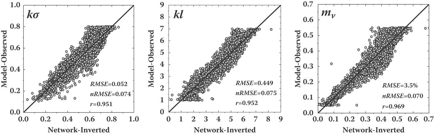
FIGURE 7.9 Retrieval of surface roughness and soil moisture from backscattering data by three inputs–three outputs DLNN configuration. Both root-mean-squared errors (RMSE) and normalized root-mean-squared errors (nRMSE) for each case are shown.
TABLE 7.4
Comparison of Inverted and Truth Data (POLARSCAT)
| Truth (POLARSCAT Data) | Inverted (Network-Inverted) | ||||
| mv | mv | ||||
| 0.949 | 2.768 | 0.142 | 0.907804 | 2.75213 | 0.141224 |
| 3.004 | 8.765 | 0.172 | 7.1636 | 12.1984 | 0.232222 |
| 0.352 | 2.617 | 0.266 | 0.346407 | 2.61012 | 0.265967 |
| 0.126 | 2.62 | 0.126 | 0.126175 | 2.62442 | 0.125997 |
| 0.352 | 2.617 | 0.14 | 0.371045 | 2.6396 | 0.14006 |
| 0.101 | 3.098 | 0.09 | 0.103238 | 3.15896 | 0.08993 |
| 1.114 | 8.287 | 0.14 | 1.20734 | 8.85712 | 0.137385 |
| 0.796 | 16.594 | 0.253 | 1.66042 | 5.38294 | 0.364186 |
| 3.004 | 8.765 | 0.172 | 3.03834 | 8.83309 | 0.172412 |
| 0.949 | 2.768 | 0.172 | 0.948958 | 2.76862 | 0.172035 |
| 6.009 | 17.529 | 0.172 | 2.69795 | 5.08291 | 0.16386 |
| 6.009 | 17.529 | 0.142 | 5.91543 | 17.6258 | 0.142792 |
| 0.352 | 2.617 | 0.266 | 0.351636 | 2.61618 | 0.266002 |
| 2.228 | 16.574 | 0.14 | 2.22803 | 16.5737 | 0.140001 |
| 0.796 | 16.594 | 0.253 | 0.797609 | 16.6051 | 0.252946 |
| 2.228 | 16.574 | 0.14 | 2.24075 | 16.5635 | 0.139998 |
| 0.398 | 8.297 | 0.253 | 0.396886 | 8.30057 | 0.252988 |
| 3.004 | 8.765 | 0.172 | 3.06484 | 8.54212 | 0.172106 |
| Error | mv | ||||
| RMSE | 1.2701 | 4.0330 | 2.987% | ||
| nRMSE | 0.2149 | 0.2705 | 0.2134 | ||
| r | 0.7706 | 0.7761 | 0.9150 | ||
7.2.3 RETRIEVAL USING BISTATIC SCATTERING COEFFICIENTS
When it comes to inversion from bistatic scattering data, we can examine the performance of using forward, backward, and full (backward plus forward), respectively. This might be practically useful since, in setting up the bistatic observation, the transmitter and receiver may be in specular or off-specular geometries. The correlation between the network-inverted result and model-observed data is shown in Figure 7.10. The inversion results were relatively close to the 1:1 line, indicating a quite-favorable correlation between the inversion and the truth data. It is worth noting that retrieval from bistatic scattering data performed better than from backscattering, especially for soil moisture inversion. Interestingly, the inversion results performed better at the forward region than in the backward region. This can also be seen quantitatively in Table 7.5, from which we can read the nRMSE being 0.060, 0.088, and 0.044 in the backward region and 0.045, 0.071, and 0.018 in the forward region for RMS height, correlation length, and soil moisture, respectively. The overall nRMSE and correlation coefficient (r) for backscattering and bistatic scatter are also given in Table 7.5. Typically, among the three surface parameters being inverted, the soil moisture tended to experience the least error, regardless of retrieval from backscattering data or bistatic scattering data. Better inversion performance seems to have been gained by the use of scattering data from the forward region. Based on this point and compared to the backscattering, it is not surprising that if we combine the scattering data from the forward and backward regions, the best retrieval accuracy in terms of nRMSE and the correlation coefficient can be obtained. This is also evident from Table 7.5, where the smaller nRMSE and higher correlation coefficient can be read as “Full” when compared to those for backscattering. It is apparently a conviction that the dynamic learning neural network as presented is able to tackle a bulky volume of data, either the training stage or operational stage, and thus achieve superior retrieval accuracy.
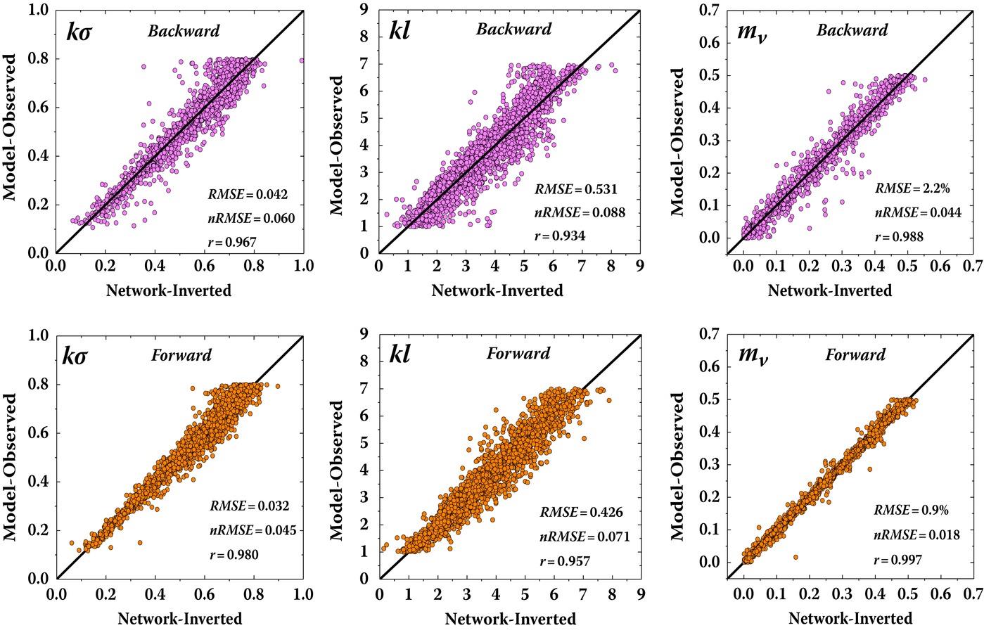
FIGURE 7.10 Retrieval performance of surface roughness and soil moisture from bistatic scattering data (four-input). Top row: backward region. Bottom row: forward region.
TABLE 7.5
DLNN Inversion Performance Using Backscattering and Bistatic Scattering
| Backscattering & Bistatic Scatter | Error | mv | |||
| Backscattering (Three-input) | nRMSE | 0.074 | 0.075 | 0.070 | |
| r | 0.951 | 0.952 | 0.969 | ||
| Bistatic scattering (Three-input) | Backward | nRMSE | 0.075 | 0.087 | 0.039 |
| r | 0.951 | 0.936 | 0.990 | ||
| Forward | nRMSE | 0.040 | 0.070 | 0.044 | |
| r | 0.985 | 0.959 | 0.988 | ||
| Full (Backward + Forward) | nRMSE | 0.058 | 0.097 | 0.042 | |
| r | 0.970 | 0.949 | 0.991 | ||
| Bistatic scattering (Four-input) | Backward | nRMSE | 0.060 | 0.088 | 0.044 |
| r | 0.967 | 0.934 | 0.988 | ||
| Forward | nRMSE | 0.045 | 0.071 | 0.018 | |
| r | 0.980 | 0.957 | 0.997 | ||
| Full (Backward + Forward) | nRMSE | 0.053 | 0.080 | 0.034 | |
| r | 0.974 | 0.945 | 0.992 | ||
There is a much higher degree of freedom to test the inversion from bistatic scattering compared to backscattering, as well as to choose the inputs, depending on the physical feasibility of the measurements. We can have measurements at the backward, forward, or combined forward and backward regions to input to the DLNN. In terms of polarization, we can have four polarizations in bistatic—two co-polarizations, two cross-polarizations, two-polarizations, or one cross-polarization. Figure 7.11 shows the retrieval performance of surface roughness and soil moisture from bistatic scattering data (three-input). The simulation test confirms the inversion performance of the neural network in terms of training and operation. From Table 7.5, we can see that the retrieval accuracy is higher using forward bistatic data than backward. The impact of polarization for bistatic cases seems not as significant as that for backscattering cases. More importantly, for the bistatic case, three inputs do not necessarily produce higher retrieval accuracy than four inputs do. It is the number of features that determine the training effectiveness and thus the retrieval accuracy. It becomes clear at this point that under the same number of inputs, inversion accuracy is higher from bistatic scattering than from backscattering. This is likely due to the fact that the bistatic scattering measurements can better separate the coupling effect of roughness and dielectric constant. For this, the sensitivity analysis given in Chapter 5 is useful for feature selection to train the neural network.
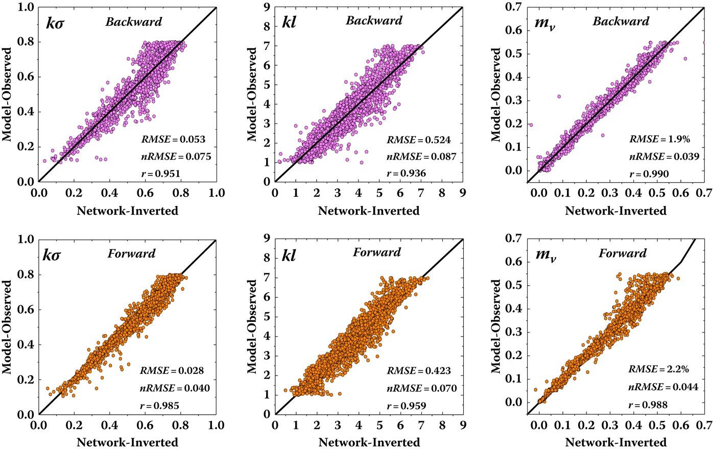
FIGURE 7.11 Retrieval performance of surface roughness and soil moisture from bistatic scattering data (three-input). Top row: backward region. Bottom row: forward region.
At this point, it is of relevance to demonstrate the retrieval of soil surface parameters from bistatic radar measurements [6,11], including roughness and moisture content, using the model-trained DLNN. A bistatic measurement facility (BMF) [11] was designed and constructed consisting of a 10 and 35 GHz polarimetric radar system for the purpose of characterizing the 3D bistatic scattering response of rough dielectric surfaces. According to, [11] a measurement with 10 GHz from a Gaussian random rough surface, with a normalized RMS height of and a normalized correlation length of , was water-soaked bricks in which the real part of the dielectric constant was 62. The incident angle and scattering angle were both set as 45°, and the scattering azimuth angle was changed from 180° to −180°. A study in [11] gave the measurements of a rough soil surface with 35 GHz using an indoor bistatic measurement facility (IBMF). At 35 GHz, the surface was assumed to be an exponentially correlated function with the normalized RMS height and correlation length being 3.28 and 29.6, respectively. The effective soil permittivity was 3.5-j0.05. The measured bistatic scattering coefficient as a function of the scattering angle (0~70°) in the backward direction () and forward direction (), and the incident angle was 20°. Another data set is taken from [6,12], where the bistatic rough dielectric surface scattering was measured at the European Microwave Signature Laboratory (EMSL) at (−10~−50°) of incidence and scattering angles with 1.5–18.5 GHz of frequency. The surface was characterized by a Gaussian correlation function with surface roughness of .
To assess the inversion performance and be more quantitative, we list the numeric results in Table 7.6, showing the measured , , and , along with the inverted data. Of the eight total test sets, the inverted results are in good agreement with the measured data. Relatively, the difference between the measured and inverted data is well within 20% error. The RMSE, nRMSE, and correlation coefficient (r) for each individual parameter, , , and , are also given. Of the three parameters, had the largest RMSE. This is consistent with our previous discussion on the measurement uncertainty of the correlation length. Nevertheless, numeric values in Table 7.6 confirm the good performance of surface parameter inversion by model-trained DLNN with inputs from bistatic radar scattering measurements.
TABLE 7.6
Comparison of Surface Parameters between Measured and Inverted by Model-Trained DLNN
| Truth (Measured) | Inverted (Network-Inverted) | Difference (Absolute) | ||||||
| 1.05 | 2.51 | 0.16 | 1.24 | 2.48 | 0.17 | 0.19 | 0.03 | 0.59% |
| 2.09 | 5.02 | 0.12 | 1.99 | 5.27 | 0.12 | 0.09 | 0.25 | 0.28% |
| 2.62 | 6.28 | 0.11 | 2.83 | 8.74 | 0.11 | 0.21 | 2.46 | 0.41% |
| 4.19 | 10.05 | 0.12 | 4.25 | 9.99 | 0.13 | 0.06 | 0.06 | 1.43% |
| 5.23 | 12.56 | 0.10 | 7.49 | 12.56 | 0.09 | 2.25 | 0.004 | 0.11% |
| 8.37 | 20.09 | 0.09 | 7.64 | 22.46 | 0.09 | 0.73 | 2.37 | 0.48% |
| 0.20 | 1.00 | 0.87 | 0.19 | 1.10 | 0.94 | 0.006 | 0.10 | 6.57% |
| 3.28 | 29.60 | 0.07 | 3.10 | 32.98 | 0.06 | 0.18 | 3.38 | 0.34% |
| mv | ||||||||
| RMSE | 0.85 | RMSE | 1.70 | RMSE | 2.41% | |||
| nRMSE | 0.10 | nRMSE | 0.09 | nRMSE | 0.03 | |||
| r | 0.95 | r | 0.99 | r | 0.99 | |||
7.2.4 COMPARISON WITH IMAGE-BASED SURFACE PARAMETER ESTIMATION FROM POLARIMETRIC SAR IMAGE DATA
The trained DLNN is now applied to the measured data acquired at L-band (1.3 GHz) from E-SAR over the floodplain of River Elbe located in North-Eastern Germany [13–15] as shown in Figure 7.12. At L-band, the spatial resolution of the single look complex data is in azimuth about 0.75 m and in the range of about 1.5 m. The data were acquired in April and August of 1997 along with two 15 km long and 3.2 km wide strips. Ground data has been collected in August 1997 over agriculture test fields with different roughness conditions. Soil moisture measurements have been performed on five different locations at each test field. The fields were viewed with incidence angle ranging from 48° to 50°. Four fields were selected due to the vegetation-covered and the choices of them were constrained by the image-based model [13] (see Table 7.7).
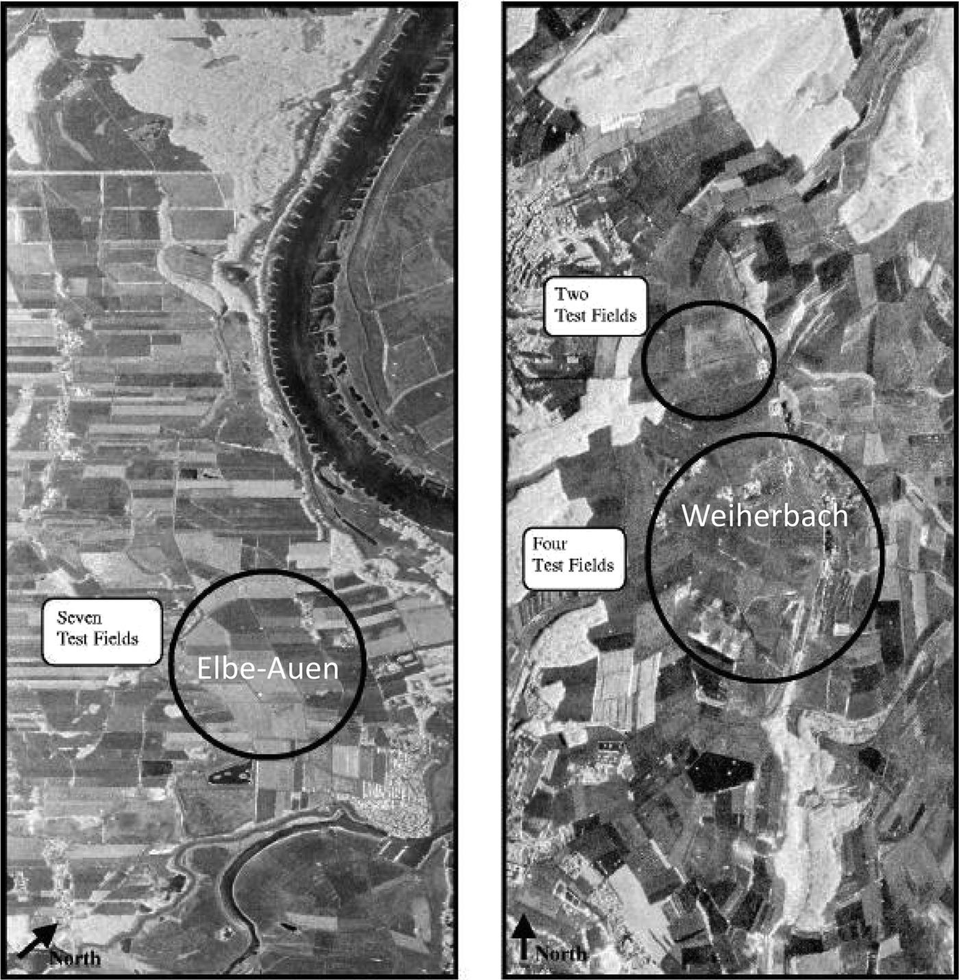
FIGURE 7.12 Total power image acquired by L-band E-SAR over the floodplain of River Elbe located in North-Eastern Germany [13].
TABLE 7.7
Ground Measurements for the Elbe-Auen Test Site
| Field ID | σ (cm) | ε′(0–4 cm) | ε′(4–8 cm) | ||
| A 5/10 | 49.20 | 1.66 | 0.45 | 10.79 | 9.28 |
| A 5/13 | 50.03 | 2.1 | 0.57 | 5.34 | 9.84 |
| A 5/14 | 49.99 | 2.77 | 0.75 | 4.51 | 10.82 |
| A 5/16 | 48.56 | 3.5 | 0.95 | 5.86 | 12.19 |
The DLNN results show that the varied inversion results using different correlated surfaces in the AIEM model. All the retrieval results (mean value for each test area) are listed in Table 7.8. First, we can see the deviation of roughness () between the inversion results and ground truth values. The largest deviation occurs for the case of field A 5/16. Gaussian correlated surface matches best for the cases. It is interesting to note that 1.5 power correlated surfaces fall in between Gaussian and exponential correlated surfaces that represent two extremes of roughness spectra in terms of their bandwidth. For horizontal roughness scale, correlation length, there is no ground truth available, the comparison is excluded. Nevertheless, the inversion outputs are listed in Table 7.8 for reference. Next, we check the retrieved dielectric constants which may be related to moisture content. It is observed that the inversion results agree well with the ground truth. To indicate this point more clearly, we plot the inverted dielectric constants by model-based DLNN and image-based [13] along with ground truth values (0–4 and 4–8 cm), as shown in Figure 7.13. The image-based results and the model-based DLNN results reasonably fall within the range of two different depths [16]. A short note is that the neural network inversion can explain more closely the observed data and hence give a good inversion result.
TABLE 7.8
The DLNN Inversion Results Using Testing the Different Correlation Functions at Different Test Sites
| A5/10 | ε′ | ||
| Gaussian | 0.51106 | 2.9856 | 8.8747 |
| Exponential | 0.36842 | 3.5310 | 10.552 |
| 1.5 Power | 0.39530 | 3.0111 | 8.6624 |
| A5/13 | ε′ | ||
| Gaussian | 0.61287 | 4.12425 | 7.6096 |
| Exponential | 0.30934 | 3.9752 | 5.5954 |
| 1.5 Power | 0.36935 | 4.0491 | 7.8188 |
| A5/14 | ε′ | ||
| Gaussian | 0.53227 | 3.7903 | 7.7906 |
| Exponential | 0.31289 | 4.0010 | 5.4194 |
| 1.5 Power | 0.35864 | 4.1336 | 10.283 |
| A5/16 | ε′ | ||
| Gaussian | 0.61799 | 3.6400 | 7.9737 |
| Exponential | 0.37857 | 3.8496 | 7.6764 |
| 1.5 Power | 0.43115 | 3.7744 | 10.025 |
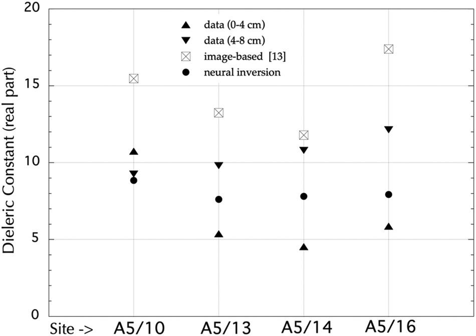
FIGURE 7.13 Retrieval versus measured dielectric constants at depths (0–4 cm) and (4–8 cm). Also included are results from image-based method [13] from four test sites: A5/10, A5/13, A5/14, A5/16.
7.3 DIRECTION ESTIMATION OF INCIDENT SOURCE: A DATA ANALYTIC EXAMPLE
Here, we estimate the source of the incident field in terms of incident angle and azimuthal angle from quad-pol radar measurements under the framework of a convolutional neural network (CNN) [3,4]. The CNN is adopted to implement the inversion of an AIEM model that relates the bistatic scattering to surface wind speed and direction. In such a case, the CNN is constructed as an inverse model. For inputs, co- and cross-polarized bistatic scattering coefficients () and scattering direction (scattering angle and scattering azimuth angle ) are selected. The outputs of the network are incident angle and incident azimuthal angel . The network training is accomplished by mapping input-output pairs that are randomly selected from the database. Note that the model predictions of the scattering represent the mean value. To generate the training samples, to be realistic, the speckle must be taken into account by using the K-distribution as discussed in the previous chapter. The radar parameters for generating training samples are given in Table 7.9.
TABLE 7.9
Radar Parameters for Generating Training Samples
| Paremeters | Range | Step Size |
| Incident Angle | 20°~70° | 5° |
| Incident Azimuth Angle | 10°~170° | 5° |
| Scattering Angle | 10°~70° | 5° |
| Scattering Azimuth Angle | 10°~170° | 5° |
| Wind Direction φ | 0°~180° | 5° |
| Frequency f | 10 GHz, 13.99 GHz | |
| Wind Speed U | 10 GHz: 3.2 m/s, 9.3 m/s, 14.5 m/s; 13.99 GHz: 5 m/s, 10 m/s, 20 m/s, 30 m/s | |
Figure 7.14 illustrates the network structure of a convolutional neural network (CNN). The retrieval result of incident direction from microwave observations with a frequency of 10 GHz arise shown in Figure 7.15, and frequency of 13.99 GHz in Figure 7.16. The root-mean-squared error (RMSE) is about 1°~2° for incident angle and 3°~4° for incident azimuthal angle, indicating that the directional estimation of the incident source is possible to achieve a satisfactory accuracy by means of CNN. Indeed, several other Backpropagation-based neural networks had been tested, such as MLP-BP, dynamic learning neural networks (DLNN), but none of them is able to give a good estimate, and most of the time, they even failed come up with outputs.
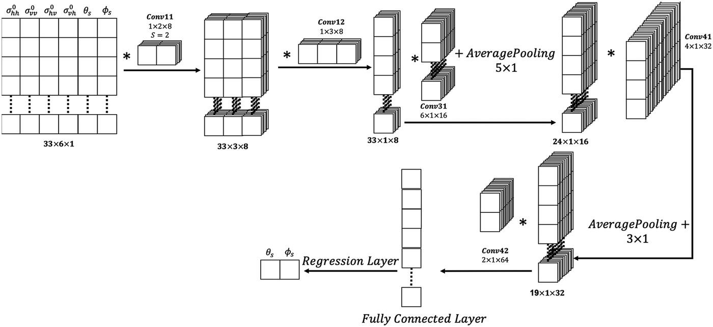
FIGURE 7.14 Network structure of a convolutional neural network (CNN).
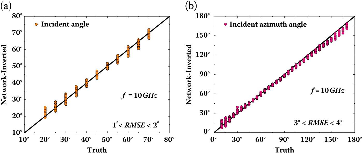
FIGURE 7.15 Correlation of wind direction between truth and reconstructed value by CNN with two frequency of : (a) inverted incident angle, (b) inverted azimuth angle.
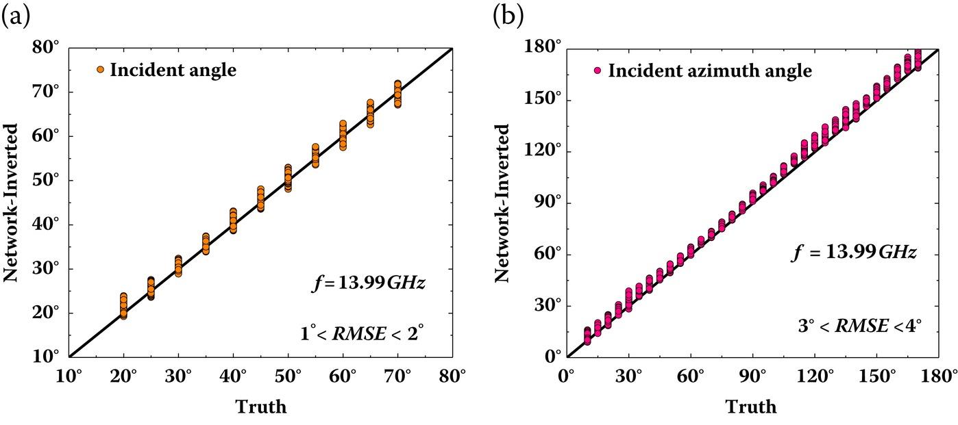
FIGURE 7.16 Same as Figure 7.15 except at frequency of 13.99 GHz.
It brings to our attention from demonstrations of the parameter retrieval that the task of rough-surface parameter (geometric and dielectric) retrieval from bistatic radar scattering data is a highly nonlinear problem. It has been shown that the use of the neural network enhances the separability for highly nonlinear boundary problems. The neural network was able to tackle the complex inversion problem with very fast learning. Experimental testing showed good performance of surface parameter inversion by the model-trained DLNN or CNN with inputs from bistatic radar scattering measurements. In the future study, through the model simulation and the proposed inversion scheme, the optimal bistatic observation configuration (in the sense of most efficient multiple inputs–multiple outputs (MIMO) to come up with high retrieval accuracy) should be investigated. It should be emphasized that, to our best understanding, real bistatic radar measurements are scant, or only taken in very limited and yet specific radar configurations (e.g., specular direction). We have demonstrated how useful bistatic data is in retrieving multiple surface parameters of interest, as compared to the backscattering data which occupies almost all of the data available, at least currently. It is therefore our objective to promote the focus more on the bistatic scattering measurements, which are shown to be powerful in inferring the surface parameters.
References
1. Hey, T., Tansley, S., Toll, K., The Fourth Paradigm: Data-Intensive Scientific Discovery, 1st edn Edition, Microsoft Research, Mountain View, CA, 2009.
2. Haykin, S. O., Neural Networks and Learning Machines, Prentice Hall, Upper Saddle River, NJ, 2008.
3. Marsland, S., Machine Learning: An Algorithm Perspective, 2nd edn Edition, Chapman & Hall/CRC, Boca Raton, FL, 2015.
4. Aggarwal, C. C., Neural Networks and Deep Learning: A Textbook, Springer, New York, 2018.
5. Oh, Y., Sarabandi, K., and Ulaby, F. T., An empirical model and an inversion technique for radar scattering from bare soil surfaces, IEEE Transactions on Geoscience and Remote Sensing, 30(2), 370–381, 1992.
6. Macelloni, G., Nesti, G., Pampaloni, P., Sigismondi, S., Tarchi, D., and Lolli, S., Experimental validation of surface scattering and emission models. IEEE Transactions on Geoscience and Remote Sensing, 38(1), 459–469, 2000.
7. Mialon, A., Wigneron, J. P., De Rosnay, P., Escorihuela, M. J., and Kerr, Y. H., Evaluating the L-MEB model from long-term microwave measurements over a rough field, SMOSREX 2006, IEEE Transactions on Geoscience Remote Sensing, 50(5), 1458–1467, 2012.
8. Zeng, J. Y., Chen, K. S., Bi, H. Y., Zhao, T. J., and Yang, X. F., A comprehensive analysis of rough soil surface scattering and emission predicted by AIEM with comparison to numerical simulations and experimental measurements. IEEE Transactions on Geoscience and Remote Sensing, 55(3), 1696–1708, 2017.
9. Fung, A. K., and Chen, K. S., Microwave Scattering and Emission Models for Users, Artech House, Norwood, MA, 2010.
10. Yang, Y., Chen, K. S., Tsang, L., and Liu, Y., Depolarized backscattering of rough surface by AIEM model. IEEE Journal of Selected Topics in Applied Earth Observations and Remote Sensing, 10(11), 4740–4752, 2017.
11. Nashashibi, A. Y., and Ulaby, F. T. MMW polarimetric radar bistatic scattering from a random surface. IEEE Transactions on Geoscience and Remote Sensing, 45(6), 1743–1755, 2007.
12. Brogioi, M., Pettinato, S., Macelloni, G., Paloscia, S., Pampaloni, P., Pierdicca, N., and Ticconi, F., Sensitivity of bistatic scattering to soil moisture and surface roughness of bare soils. International Journal of Remote Sensing, 31, 4227–4255, 2010.
13. Hajnsek, I., Pottier, E., and Cloude, S. R., Inversion of surface parameters form polarimetric SAR, IEEE Transactions on Geoscience and Remote Sensing, 41(4), 727–744, 2003.
14. Hajnsek, I., Jagdhuber, T., Schon, H., and Papathanassiou, K. P., Potential of estimating soil moisture under vegetation cover by means of PolSAR. IEEE Transactions on Geoscience and Remote Sensing, 47(2), 442–454, 2009.
15. Jagdhuber, T., Hajnsek, I., Bronstert, A., and Papathanassiou, K. P., Soil moisture estimation under low vegetation cover using a multi-angular polarimetric decomposition, IEEE Transactions on Geoscience and Remote Sensing, 51(4), 2201–2214, 2012.
16. Lee, H. W., Chen, K. S., Lee J. S., Shi, J. C., Wu, T. D., and Hajnsek, I., A comparisons of model based and image-based surface parameters estimation from polarimetric SAR. In Proceedings of the 2005 IEEE International Geoscience and Remote Sensing Symposium, 2005. doi:10.1109/igarss.2005.1526460.