5 Sensitivity Analysis of Radar Scattering of Rough Surface

Sensitivity analysis (SA) of electromagnetic waves scattering from a randomly rough surface is pivotal in the field of remote sensing of surface geometrical and dielectric parameters [1–3]. It has been routine to retrieve the geophysical parameters of interest, such as soil moisture and roughness, from the radar scattering measurements [4–7], based on analyzing the sensitivity of the scattering behavior and mechanisms. By capturing the scattering patterns, one could effectively avoid undesired parameters, while devising a means to retrieve the parameters of interest. Knowing how the variation in the model outputs attributes to the variation of the inputs is critical [8]. SA can be on local and global scales [9]. Local SA is a gradient-based method that analyzes only one parameter in a model at a time while fixing all of the remaining parameters to their nominal values [9]. Local SA is simple and computationally efficient. However, it fails to quantify the interactions among all the parameters of interest; hence it may not be a good choice for the nonlinear and non-monotonic model [10]. Global SA, on the other hand, considers the mutual coupling among all the parameters within their ranges. That is, all the parameters in a model are simultaneously analyzed in global SA.

Among the global SA methods, the extended Fourier amplitude sensitivity test (EFAST) [11–16] and entropy-based sensitivity analysis (EBSA) [17], are two common methods. EFAST is one of the most popular methods for SA and is applicable to nonlinear and non-monotonic models, and can quantify the parameter interaction effects as well. Besides, to preserve the maximum information content of the parameters of interest, which are transferred from inputs to outputs of the radar response, EBSA has been proposed to characterize the information content in terms of communications theory, to quantitatively and objectively evaluate the information of the sensor configurations, and to evaluate observational uncertainty that is associated with parameter sampling [18]. In this chapter, we will focus on these two methods and show the numerical results.

5.1 EXTENDED FOURIER AMPLITUDE SENSITIVITY TEST (EFAST)

EFAST, a variance-based, is developed based on FAST and Sobol [19]. The FAST method offers a high-efficiency sampling method that is based on a suitably defined search curve. However, it can only calculate the “main effect” contribution of each input parameter to the model outputs. Thus, it cannot identify the parameter interaction effects on the model outputs. The Sobol method is capable of computing higher interaction terms but is computationally expensive since it adopts Monte Carlo sampling. EFAST fuses the strengths of FAST and Sobol to obtain the total and the main sensitivity indices (SIs) of each input parameter.

The EFAST algorithm mainly includes two steps: sampling and SIs computation. The random sample is first generated by converting the multidimensional parameter space into a 1-D space via a transformation function. The sample size N_s is calculated by using the largest sampling frequency $ω_{\max}$ and the number of exploring curves N_r as

$N_{s} = (2 M ω_{\max} + 1) N_{r}$ (5.1)

where M is a interference factor. To ensure a reasonable sampling density, Saltelli et al. [11] suggested some constraints for the parameters: M = 4, $ω_{\max} \geq 8$ and $16 \leq ω_{\max} / N_{r} \leq 64$ . Once $ω_{\max}$ and N_r are fixed, the number of random samples can be determined.

The second step is to calculate the SIs for each model input, which is expressed by two indices: the main sensitivity index (MSI) and the total sensitivity index (TSI), as

$M S I_{i} = \hat{V a r_{i}} (Y) / \hat{V a r} (Y)$ (5.2)

$T S I_{i} = 1 - \hat{V a r_{(- i)}} (Y) / \hat{V a r} (Y)$ (5.3)

$\sum_{j = 1, j \neq i}^{n} S_{i, j} = T S I_{i} - M S I_{i}$ (5.4)

where $\hat{V a r_{i}} (Y)$ is the estimated conditional variance of the ith factor, $\hat{V a r_{(- i)}} (Y)$ is the estimated conditional variance except for the ith factor, and $\hat{V a r} (Y)$ is the variance of output $Y$ . $MS I_{i}$ is the main (or first-order) sensitivity index of the ith factor, which represents the main contributions of each input parameter to the variance of the model output, and $TS I_{i}$ is the total (including higher-order effects) sensitivity index of the ith factor, which considers the interactions among parameters. If $MS I_{i}$ differs from $TS I_{i}$ , interactions between parameters exist. Both $MS I_{i}$ and $TS I_{i}$ range between 0 and 1; higher $MS I_{i}$ and $TS I_{i}$ values suggest more important effects of the ith factor on the output. In Equation (5.4), $S_{i, j}$ represents the parameter interaction. For a detailed description and mathematical derivations of EFAST, readers are referred to [9], [11].

5.2 ENTROPY-BASED SENSITIVITY ANALYSIS (EBSA)

For a random rough surface, the scattering response varies nonlinearly with the surface conditions. There exists a well-known problem of uniqueness in the radar response measurement, because of the complex wave-target interactions, as well as uncertainty sources, such as the random characteristics of the rough surface and noise-corrupted radar echoes [20, 21]. It has been proven that, for the backscattering from a randomly rough surface, the Shannon entropy is a good indicator of the sensitivity of radar response to surface parameters because it not only reflects the probabilistic distribution of scattering coefficient but also the deviation [18]. In EBSA, more information on scattering behavior can be preserved through evaluating detailed parameter sensitivities, predicting the scattering signal saturation, estimating the advantage of multi-polarization and multi-angle, and identifying less significant variables. It is convinced that EBSA offers richer details of scattering sensitivity. The procedure EBSA composes of three steps: sampling input data, computing Shannon entropy (SE) and performing sensitivity analysis.

Sampling input data: generating sufficiently ample normally distributed random samples of surface parameters and bistatic configurations. The range of parameters includes surface roughness, dielectric constant, and bistatic configuration.
Computing Shannon entropy: feeding the generated samples into the AIEM model to compute the scattering coefficients and the corresponding Shannon entropy SE [22]:

$S E = E [H (b)] = E [- \ln (P (b))]$ (5.5)

where E is an expected value operator, and H is the Hartley’s information content of observation $b$ , and P is the probability density function (pdf), which can be estimated by kernel density method with a Gaussian kernel [23].
Performing sensitivity analysis: tackling the signal changes in the bistatic scattering pattern by a varying one single parameter with the other parameters remaining unchanged to analyze the radar signal sensitivity to the surface roughness, moisture content, and bistatic configuration at both co- and cross-polarizations are examined.

To assess the performance of SE as well as scattering behavior, we may look into some distribution parameters, including skewness $γ$ , kurtosis $κ$ , and standard deviation σ_std.

$γ = \frac{E [{(x - μ)}^{3}]}{{σ_{s t d}}^{3}}$ (5.6)

$κ = \frac{E [{(x - μ)}^{4}]}{{σ_{s t d}}^{4}} - 3$ (5.7)

$σ_{s t d} = \sqrt{(\sum_{i = 1}^{n} {(x_{i} - \bar{x})}^{2}) / n}$ (5.8)

where μ is the mean of the random variable x, and σ_std measures statistical dispersion, and $γ$ measures the asymmetry of the data around the sample mean, and $κ$ indicates how outlier-prone a distribution would be. Thus, $γ$ and $κ$ , equal to zero for a normal distribution. If $γ$ is negative-valued, the data are spread out more to the left of the mean than to the right. Distributions that are more outlier-prone than the normal distribution have a positive value of $κ$ , with a negative value of $κ$ indicating distributions that are less outlier-prone than the normal distribution.

5.3 MONOSTATIC VS. BISTATIC SCATTERING PATTERNS

5.3.1 MONOSTATIC SCATTERING PATTERNS

5.3.1.1 Distribution Response of the Backscattering Coefficient

Figure 5.1 is a scattering coefficient distribution with the normal disturbed rough surface parameter as inputs. The exponential correlation function is used at an incident angle of 45°. In the figure, we can see that, for dry and smooth surface, the scattering coefficient remains normal distributed. With increasing surface roughness and moisture content, the behavior of the rough surface scattering is not normally distributed, as is frequently assumed. It is more likely to be Beta distribution, as shown in Figure 5.2. This disagreement can be described by the departures of the $γ$ and $κ$ of returns from normal distribution counterparts. Moreover, we can see that, compared to the surface with varying $k l$ and $m_{v}$ , the scattering response deviation is more obvious when varying $k σ$ . Finally, it can be observed that the HH-polarized distribution response is generally similar, but not exactly the same, as the VV-polarized ones.

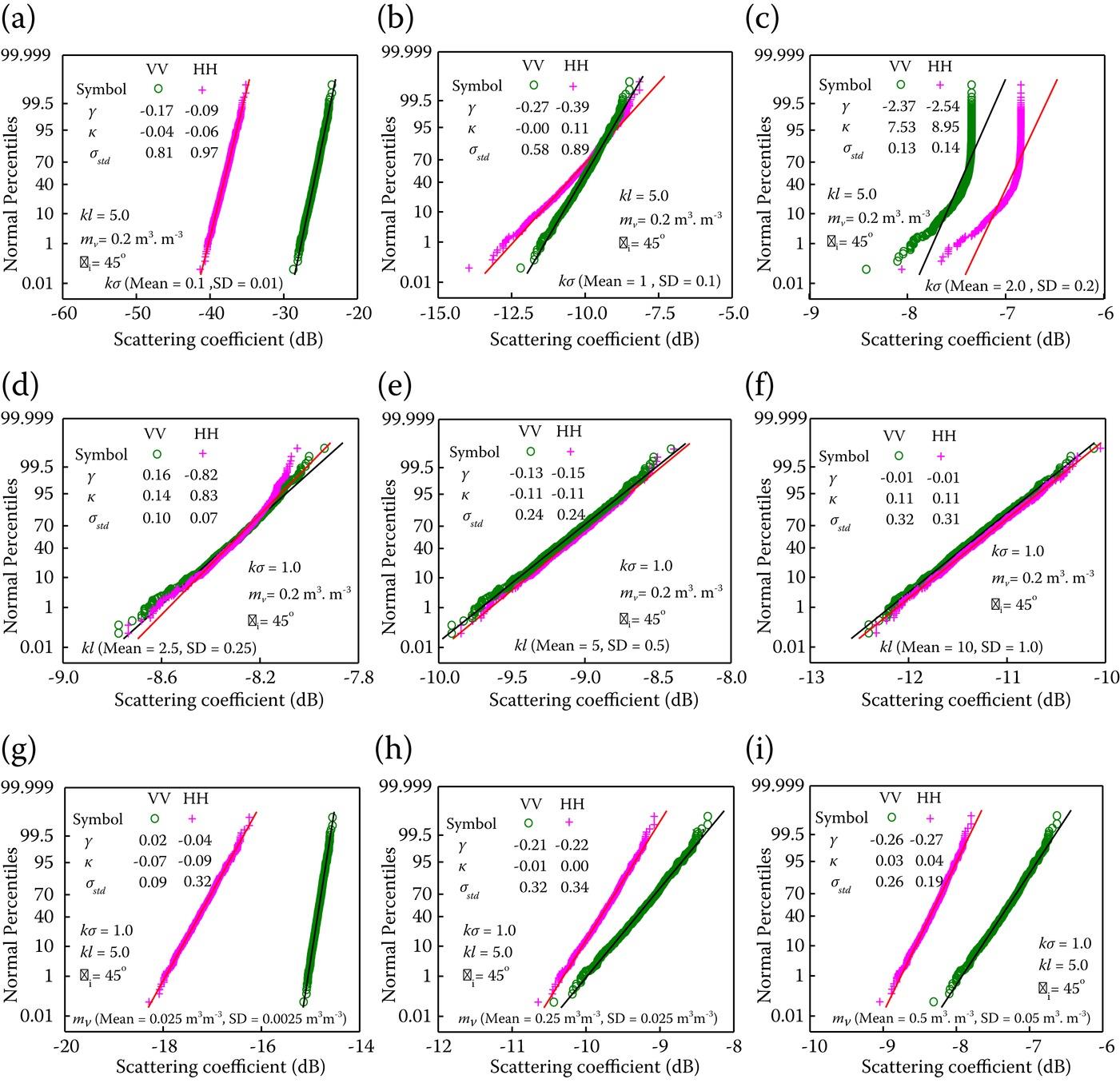
**FIGURE 5.1** Probability of the scattering coefficient with normal distributed input surface parameters of (**a–c**) $k σ$ ; (**d–f**) $k l$ ; and (**g–i**) $m_{v}$ , at the incident angle of 45°. The solid line is the reference line for a normal distribution fit. (a, d, g) small $k σ$ , $k l$ , and $m_{v}$ ; (b, e, h) medium $k σ$ , $k l$ , and $m_{v}$ ; and (c, f, i) large $k σ$ , $k l$ , and $m_{v}$ . The parameters on upper left of the figures show the distribution of the scattering coefficients, while on the bottom are the input parameters.

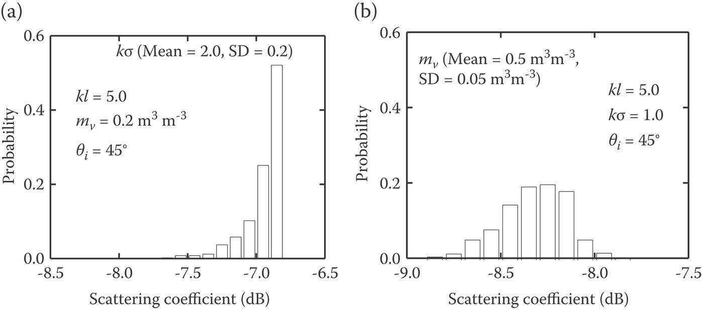
**FIGURE 5.2** Probability distribution response of backscattering for rough surface with (a) great roughness; and (b) high water content.

5.3.1.2 SA by Information Entropy

Figure 5.3 is a volumetric slice of SE with three key surface parameters, namely, $k σ$ , $k l$ , and $m_{v}$ in the x, y, z directions, respectively. In the figure, we observe that the entropy related to the HH polarization is generally similar to that of VV polarization. Moreover, the backscattering signals were found to be more sensitive to $k σ$ than to $m_{v}$ and $k l$ . Those results are highly consistent with those by other methods, such as EFAST methods. The consistency between the different models indicates again the feasibility of the proposed entropy-based method in SA.

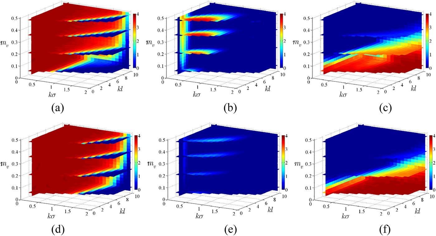
**FIGURE 5.3** SE response to rough surface when varying: (**a, d**) $k σ$ ; (**b, e**); and (**c, f**) $m_{v}$ at a polarization of: (**a–c**) VV; and (**d–f**) HH. The incident angle is 45° and the frequency is 1.26 GHz. Normal distribution disturbances were added to the input parameters, with σ equal to 1% of the maximum of the corresponding surface parameters. As an example, SD is set to 0.02, 0.1, and 0.005 $m^{3} \cdot m^{- 3}$ when varying: (**a, d**) $k σ$ ; (**b, e**) $k l$ ; and (**c, f**) $m_{v}$ , respectively.

Note that, compared to other SA methods, the entropy-based method provide more specific and detailed parameter sensitivity under various rough surface conditions, while there is always only single SA data for global SA or limited data for local SA. Therefore, the proposed method can give us more insight into the scattering behaviors of the rough surface and, thus, ensure better use of microwave scattering data in surface monitoring. Another interesting finding is that it is easy to determine the saturation point of backscattering signals in the form of rapidly decreasing entropy. For example, it can be seen that backscattering signals tend to saturate for a rougher surface, and wet soil prompts the saturation.

5.3.2 BISTATIC SCATTERING PATTERNS

To explore the distribution response of the bistatic scattering coefficient, we start with an intermedium roughness ( $k σ = 1.0$ ), with the remaining parameters being fixed to ( $k l = 5.0, m_{v} = 0.2 m^{3} m^{- 3}$ ). Figure 5.4 shows the hemispherical plots of the standard deviation σ_std and their $SE$ values at an incident angle of 50°, for both cross- and co-polarizations. In this plot, the left and right halves correspond to the backscattering and forward scattering direction, respectively, and the horizontal and vertical axes represent the incident and cross planes, respectively. It must be noted that, the exponential correlation function is used because of its good representation of natural surface conditions. Regarding σ_std, a stronger co-polarization σ_std closes to the specular region, a smaller σ_std in the backward region, and the appearance of a minimum HH-polarized σ_std around the cross-plane (the vertical axis), the apparent locations of the VV minima along the arc, and a nearly disappearing cross-polarized σ_std in the incidence plane (the horizontal axis). Accordingly, a high SE always corresponds to small deviations from a normal distribution and a large standard deviation σ_std. Moreover, the overall cross- and co-polarized distribution responses are generally similar, despite not being exactly the same. It is interesting to find that the greatest scattering sensitivity to $k σ$ is found in the backward direction, and the scattering signals always saturate in the forward direction.

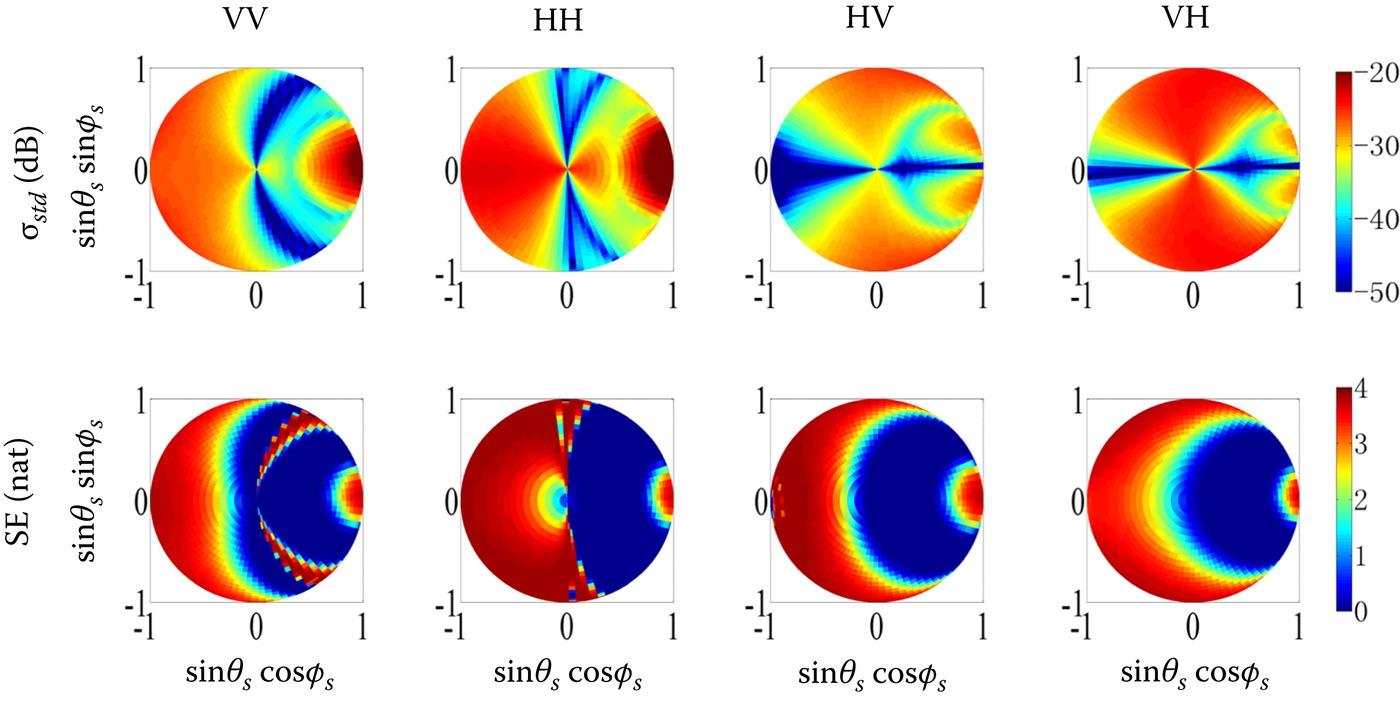
**FIGURE 5.4.** Hemispherical plots of the standard deviation σ_std and the corresponding Shannon entropy ( $SE$ ) with the normally disturbed $k σ$ as the input: VV (first column); HH (second column); HV (third column); VH (fourth column), at θ_I = 50°, with kl = 5.0, and $m_{v} = 0.2 m^{3} m^{- 3}$ .

Figure 5.5 shows the hemispherical plots of the standard deviation σ_std, and their $SE$ values at an incident angle of 50°, for both cross- and co-polarizations. The scattering response to $kl$ is found to be quite different from that of $k σ$ . A number of significant SE values are found at large scattering angles in the forward and backward directions, for both cross- and co-polarizations, and around the perpendicular planes for co-polarizations. Thus, the effect of correlation length at those directions should be carefully considered in bistatic observation, whereas it has almost no effect on mono-static observation for most rough surface conditions. Moreover, there appears to be a new, nonsensitive scattering response region in the backward direction with small σ_std, such as regions at small scattering angles for VV polarization and around the perpendicular scattering plane for HH polarization.

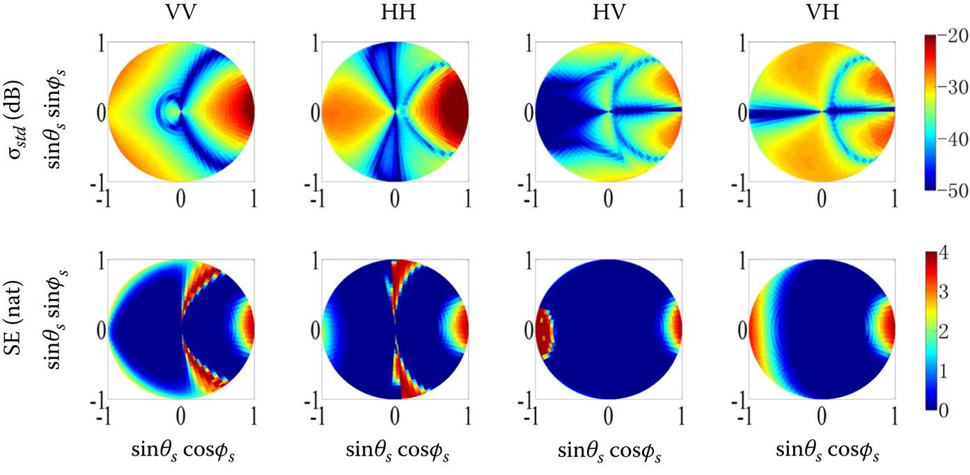
**FIGURE 5.5** Hemispherical plots of the standard deviation σ_std and the corresponding Shannon entropy ( $SE$ ) with the normally disturbed $kl$ as the input: VV (first column); HH (second column); HV (third column); VH (fourth column), at θ_i = 50°, with $k σ = 1.0$ , and $m_{v} = 0.2 m^{3} m^{- 3}$ .

Figure 5.6 shows hemispherical plots of the bistatic scattering coefficient for surface with normally disturbed water content. In general, the scattering sensitivities to $m_{v}$ are different for all four polarizations. For VV polarization, scattering in the forward direction is more sensitive than in the backward direction. For the HH polarization, the behavior is the opposite.

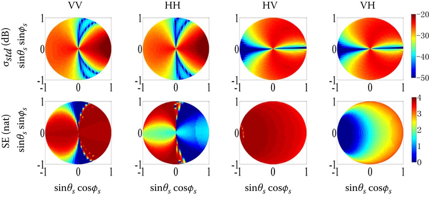
**FIGURE 5.6.** Hemispherical plots of the standard deviation σ_std, and the corresponding Shannon entropy ( $SE$ ) with the normally disturbed $m_{v}$ as the input: VV (first column); HH (second column); HV (third column); VH (fourth column), at θ_i = 50°, with $kl = 5.0$ , and $k σ = 1.0$ .

5.4 DEPENDENCES ON RADAR PARAMETERS

5.4.1 SENSITIVITY TO INCIDENT ANGLE

Figure 5.7 shows the entropy as a function of the incident angles. The SE decreases first and then increases, and the smallest entropy is always found around the small incident angles for a smooth surface, and it shifts toward a greater incident angle for rougher cases. This finding indicates that, for roughness sensing, the backscattering observation at greater incident angles is preferable for a smooth surface, while smaller incident angles for rough surfaces, to retain the maximum information. The distribution of $m_{v}$ is notably different from that of $k σ$ . The SE curve with varying $k σ$ is monotone, and the scattering signal saturates more quickly for a more wet surface. The above results are based on VV polarization. Similar behavior with HH polarization is observed.

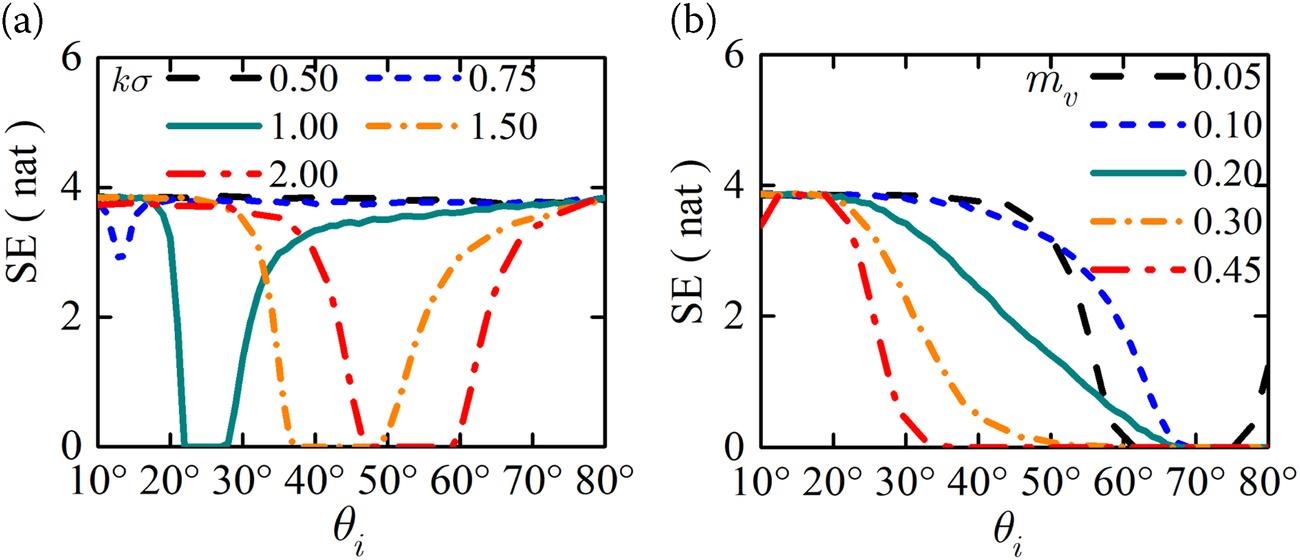
**FIGURE 5.7** SE as a function of incident angles for varying (a) normalized rms height $k σ$ ( $k l = 5.0$ , $m_{v} = 0.2 m^{3} \cdot m^{- 3}$ ) and (b) moisture content $m_{v}$ ( $k σ = 1.0, k l = 5.0$ ).

5.4.2 SENSITIVITY TO POLARIZATION

Two sets of simulation data with dual-polarization are combined (i.e., the polarization ratio and the polarization difference), as given in Figure 5.8. The figure shows that dual-polarization is expected to provide some improvements in estimating the moisture content compared to single-polarized measurements by reducing the scattering coefficient saturation for rough and wet surfaces, which is a problematic issue in surface parameter retrieving.

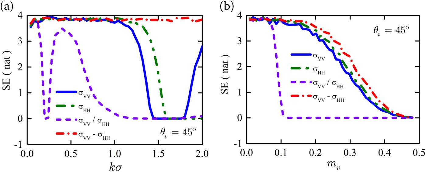
**FIGURE 5.8.** SE of single- and dual-polarization for varying (a) normalized rms height $k σ$ ( $k l = 5.0, m_{v} = 0.2 m^{3} \cdot m^{- 3}$ ) and (b) moisture content $m_{v}$ ( $k σ = 1.0, k l = 5.0$ ) at θ_i = 45°.

5.4.3 SENSITIVITY TO MULTI-ANGLE

For multi-angle observations, we investigate the SE response of two angles (θ_i = 30°, 45°), and three angles (θ_i = 30°, 45°, 50°) in simulations, as shown in Figure 5.9. Note that only varying the roughness $k σ$ and moisture content $m_{v}$ were considered because the scattering response to $k l$ is comparatively less sensitive. The figure shows that a multi-angle observation can help to address the issue of the scattering signal saturation for wet and rough surfaces, which is similar to the using dual-polarization. It is interesting to note that for multi-angle, which is the combination of backscattering coefficients at two incident angles (σ_VV(30°)/σ_VV(45°)), the SE is sensitive to $k σ$ but not to $m_{v}$ , while the combination of three angles

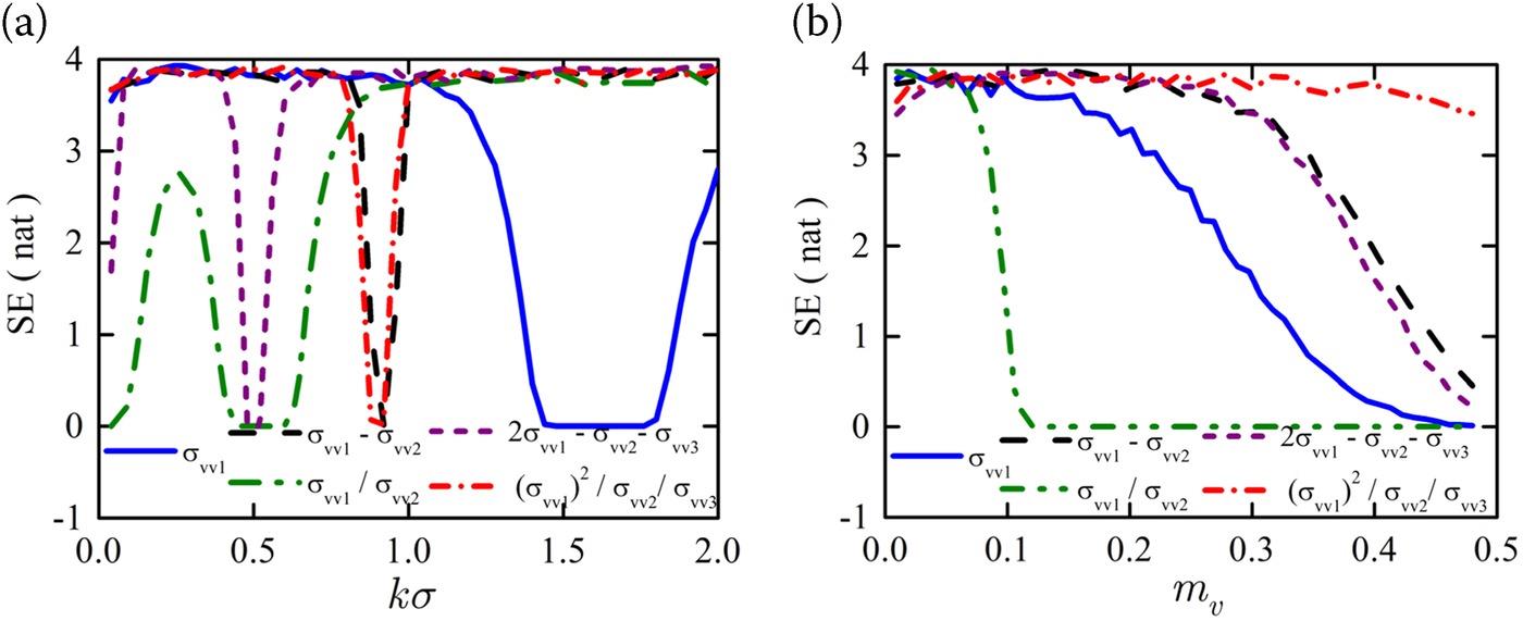
**FIGURE 5.9.** SE of the single and multi-angle when varying (a) normalized rms height $k σ$ ( $k l = 5.0, m_{v} = 0.2 m^{3} \cdot m^{- 3}$ ) and (b) moisture content $m_{v}$ · $k σ = 1.0, k l = 5.0$ . σ_VVi is the VV-polarized scattering coefficient with the incident angle ϑ_i = 30°, 45°, 50°.

(σ_VV(30°))²/(σ_VV(45°)σ_VV(50°)) shows sensitivity to both $k σ$ and $m_{v}$ . This finding implies that one can use the ratio between the values of the backscatter data at two angles to estimate the roughness while assigning the soil moisture at a constant value. The soil moisture can then be estimated based on the ratio of the three backscatter values using the estimated roughness. Note that there is an obvious SE dip for a multi-angle observation due to the almost equal scattering coefficients of those angles.

To indicate quantitatively the effect of the angular combination, we compared the sensitivity of bistatic scattering observation, including single input–single output (SISO) and single input–multiple output (SIMO), with a comparison of the mono-static observation in Figure 5.10, which shows the effect of angular combination of bistatic observation on sensitivity to $k σ$ and $m_{υ}$ , with a comparison of mono-static observation for VV polarization. The parameters are given in Table 5.1. The results show that the angular combination can greatly improve the information of interest parameters of the rough surface.

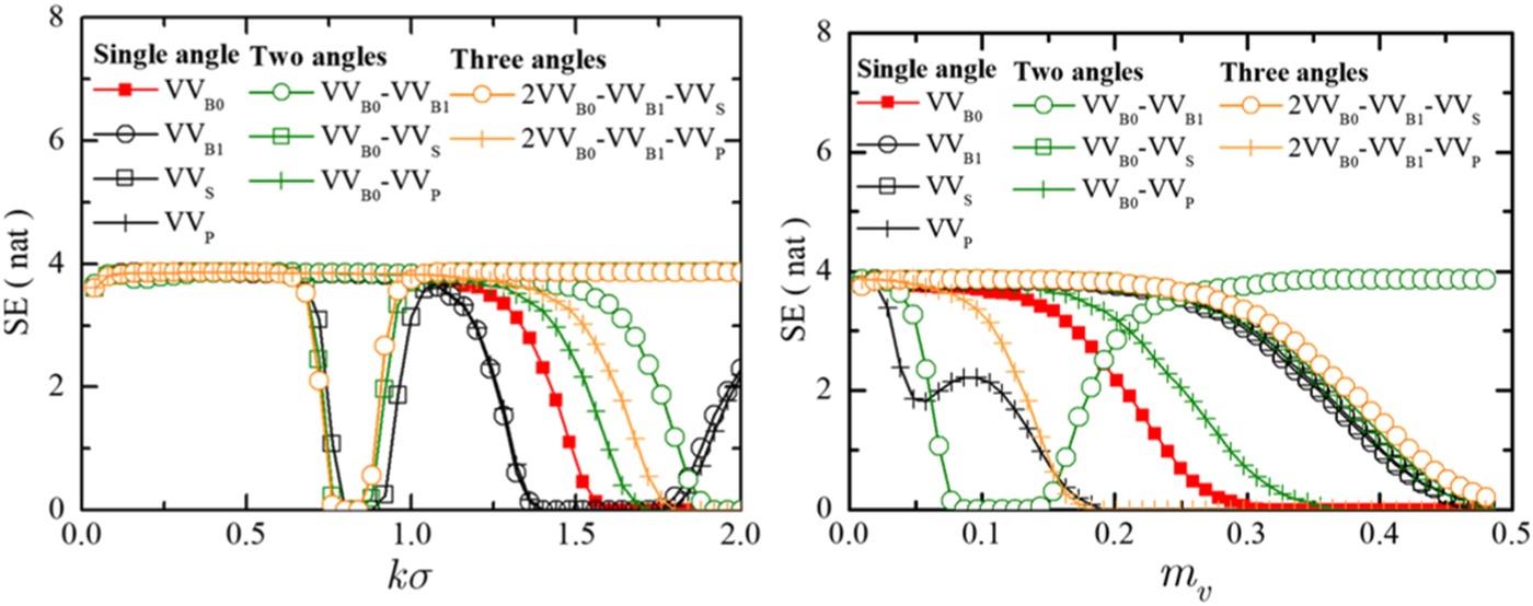
**FIGURE 5.10.** SE as a function of (a) $k σ$ , with $m_{υ} = 1$ and $m_{υ} = 0.2 m^{3} \cdot m^{- 3}$ and (b) $m_{υ}$ , with $k σ = 1$ and $m_{v} = 0.2 m^{3} m^{- 3}$ ·VV_n, n = B₀, B₁, S, P, B₀ and B₁ are backscattering observations with (ϑ_s, ϕ_s) equal to (50°, 180°) and (40°, 180°), respectively, S shows the observation in the specular scattering plane (50°, 0°), and P in perpendicular plane (50°, 90°) at θ_I = 50°.

Table 5.1 Angular Combination of Bistatic Observations

Type		Receiving Direction	Receiving Angle
mono-static	SISO	Backward	(50°, 180°)	B0
	SISO	Backward	(40°, 180°)	B1
	SISO	Perpendicular	(50°, 90°)	P
	SISO	Specular	(50°, 0°)	S
	SIMO	Backward	(50°, 180°), (40°, 180°)	B0, B1
Bistatic	SIMO	Backward, Perpendicular	(50°, 180°), (50°, 90°)	B0, P
	SIMO	Backward, Specular	(50°, 180°), (50°, 0°)	B0, S
	SIMO	Backward, Perpendicular	(50°, 180°), (40°, 180°), (50°, 90°)	B0, B1, P
	SIMO	Backward, Specular	(50°, 180°), (40°, 180°), (50°, 0°)	B0, B1, S

Note: The incident angles are (50°, 0°). SISO means single input and single output observation; SIMO single input and multi-output.

5.5 DEPENDENCES ON SURFACE PARAMETERS

Three key parameters, i.e., soil moisture (m_v), root mean square height (σ), and correlation length (l), which exert significant influence on radar signals are selected, and their distributions and ranges in the AIEM model simulation are listed in Table 5.2. It is known that the ranges of the parameters impact the sensitivity indices and importance ranking of the parameters, which depends on the available information and the goal of the study. In some regional-dependent studies (e.g., [12], [24]), the ranges of the parameters are determined from local measurements. We may want to cover all the cases that can represent natural surface conditions (e.g., from a very smooth or dry surface to a rough or wet surface). It is a common practice to analyze the parameters covering a wide range of conditions [25].

Table 5.2 Input Parameters and Their Distributions and Ranges in the AIEM Scattering Model

Parameter (unit)	Definition	Distribution	Range
m_v (m³ m⁻³)	soil moisture	uniform	0.01~0.5
σ (cm)	RMS height	uniform	0.1~3
l (cm)	correlation length	uniform	2.5~35

We conduct SA tests on the whole upper half-space with 0° ≤ θ_s ≤ 60° and 0° ≤ ϕ_s ≤ 180° for the incident angles of 40°. It is known that bistatic scattering behavior is controlled by the surface correlation function together with σ and l, for characterizing surface roughness. Three commonly used correlation functions including exponential, Gaussian, and 1.5-power, are selected. Since the cross-polarized scattering coefficient is more sensitive to the volume scattering, it is often used to detect the growth of vegetation rather than soil moisture [26]–[27]. We calculate the SIs (TSI and MSI) and their difference (parameter interaction effects) for soil moisture, RMS height, and correlation length with respect to the bistatic scattering coefficient at both HH and VV polarizations respectively. Since the distributions of MSI and TSI on the whole upper half-pace are similar, we simply present the results of MSI for the three parameters.

5.5.1 SENSITIVITY TO SOIL MOISTURE

Figure 5.11 displays the distribution of MSI of soil moisture that is associated with VV-polarized and HH-polarized bistatic scattering coefficients on the whole upper half-space as a function of scattering angle θ_s and azimuth angle ϕ_s for incident angles of 40° with different correlation functions respectively. For VV polarization, as shown in Figure 5.11(a–c), the maximum sensitivity to soil moisture is in the forward direction regardless of incident angles and correlation functions. It was found that the bistatic scattering signals at or near an orthogonal configuration are most sensitive to soil moisture, and a small incident angle at VV polarization was suggested for SAOCOM to infer soil moisture [28]. However, the orthogonal or quasi-orthogonal directions may pose a problem because the co-polarized radar signals in these regions are small and maybe close to the receiver noise floor (i.e., the lowest measurable scattering coefficient due to system noise). Thus, from a practical point of view, observations near the cross-plane are not suggested [25]. Moreover, we can see there is always an obvious high-sensitivity point for MSI of soil moisture and a corresponding low-sensitivity point for RMS height near the cross-plane, regardless of the correlation function, when the scattering angle is equal to the incident angle. This phenomenon may be caused by the combined effects of both geometric parameters and ground surface conditions on radar signals, and may also be related to the “dip” feature in the azimuthal plane. Since the co-polarized radar signals in these regions are small, it is challenging to discriminate the return signals at such a narrow-angle. Meanwhile, from Figure 5.11(a–c) we can observe that correlation function does not have much impact on the bistatic sensitivity pattern of soil moisture, which leads to similar distributions of MSI of soil moisture under different correlation functions. As shown in Figure 5.11(d–f), we can see that the bistatic sensitivity pattern of soil moisture at HH polarization is generally different from that at VV polarization, though with a few similarities. An intermediate incident angle (e.g., 40°) is recommended if HH polarization is used to estimate soil moisture. However, we can clearly see that the MSI values of soil moisture at HH polarization are generally small compared with those at VV polarization on the whole upper half-space, which is even more evident for a Gaussian-correlated surface. This finding is confirmed in more detail based on a global SA analysis, which demonstrates that bistatic VV polarization is preferable to HH polarization for soil moisture estimation. More numerical results and discussions can be found in [29].

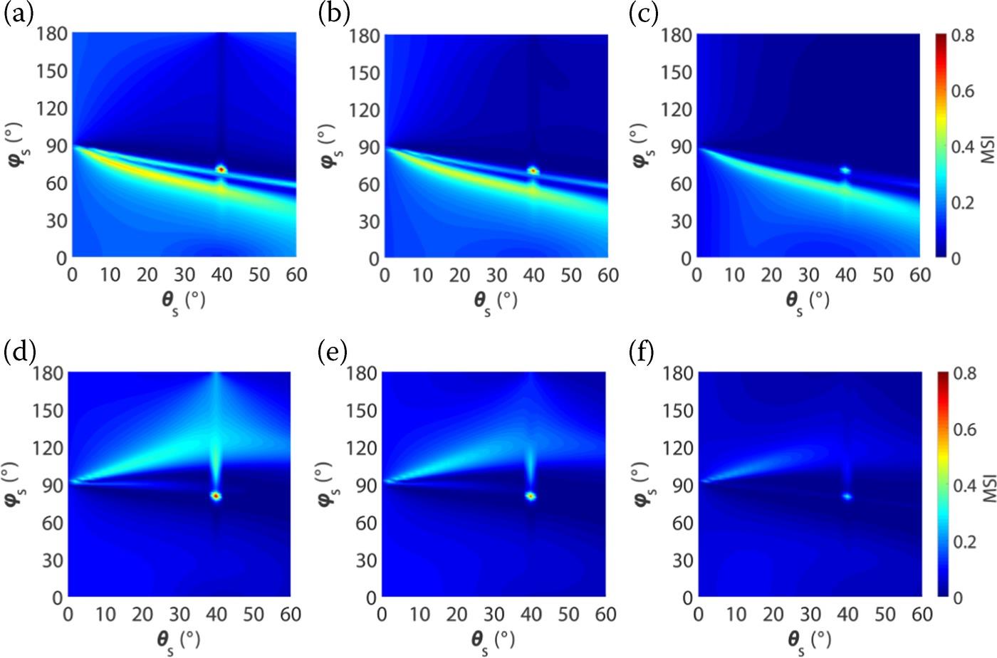
**FIGURE 5.11** MSI of soil moisture derived from VV-polarized (top row: (**a–c**)) and HH-polarized (bottom row: (**d–f**)) scattering coefficients as a function of scattering angle θ_s and azimuth angle ϕ_s at L-band for incident angles, θ_i, of 40° with different correlation functions from left to right, i.e., (**a, d**) exponential, (**b, e**) 1.5-power, and (**c, f**) Gaussian.

In what follows, we examine the interactions between m_v, σ, and l and other parameters as functions of scattering angle θ_s and azimuth angle ϕ_s, with incident angles θ_i of 40° with exponential, 1.5-power and Gaussian correlation functions. We first present the results of VV polarization for soil moisture in Figure 5.12(a–c) and HH polarization in Figure 5.12(d–f). We can see that for all three parameters, the interaction effects are generally small and close to zero for most parts of the whole upper half-space. That is, in these scattering geometries, the first-order (MSI) and total-order (TSI) sensitivity indices are almost equal. Figure 5.12(a–c) displays the interactions of soil moisture with other parameters (e.g., soil moisture with RMS height, soil moisture with correlation length, and soil moisture with RMS height and correlation length). We see that the maximum interaction effects are very close to the cross-plane. As shown in Figure 5.12(d–f), for HH polarization, the difference between TSI and MSI for all the three parameters is very small on the whole upper half-space at L-band [29]. It was found that the interactions are smallest at L-band and increase as the frequency increases. Since it is almost impossible to decompose these interactions from radar signals that introduce uncertainties into soil moisture retrieval, observations at L-band for soil moisture estimation are suggested.

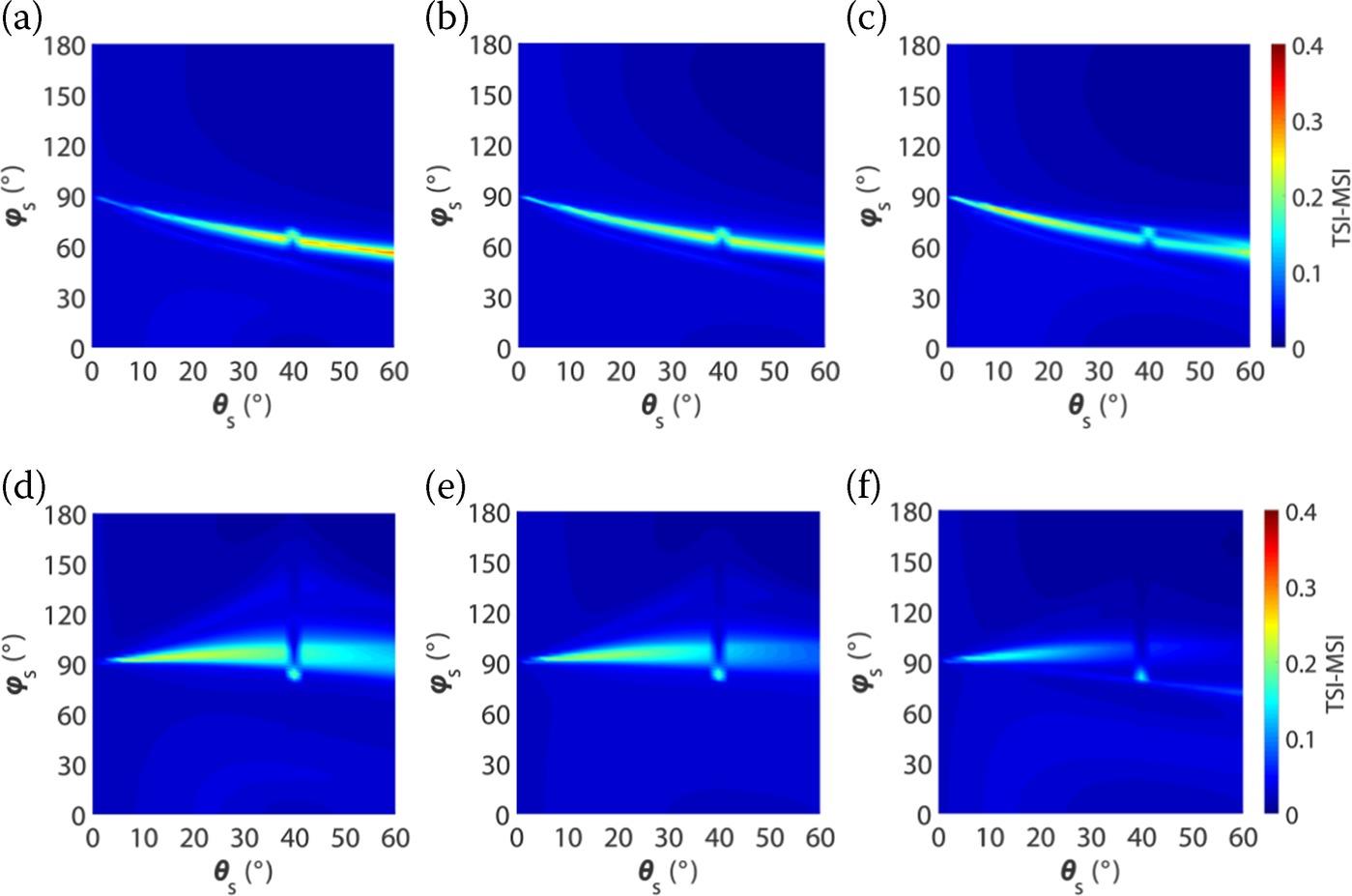
**FIGURE 5.12** TSI-MSI (the difference between TSI and MSI) of soil moisture derived from VV-polarized (top row: (**a–c**)) and HH-polarized (bottom row: (**d–f**)) scattering coefficients as a function of ϑ_s and ϕ_s at L-band for incident angles ϑ_i of 40° with correlation functions from left to right, i.e., (**a, d**) exponential, (**b, e**) 1.5-power, and (**c, f**) Gaussian.

5.5.2 SENSITIVITY TO RMS HEIGHT

Figure 5.13 displays the distribution of MSI of RMSH that are associated with VV-polarized and HH-polarized bistatic scattering coefficients on the whole upper half-space as a function of scattering angle θ_s and azimuth angle ϕ_s for incident angles θ_i of 40° with different correlation functions respectively. For VV polarization, as shown in Figure 5.13(a–c), we can see that the RMSH exerts a significant influence on radar signals in a bistatic mode. Note that the sensitive zones of RMSH are largest for exponentially correlated surfaces and smallest for Gaussian-correlated surfaces. Moreover, we can see there is always an obvious low-sensitivity point for RMSH near the cross-plane, regardless of the correlation function, when the scattering angle is equal to the incident angle. This phenomenon may be caused by the combined effects of both geometric parameters and ground surface conditions on radar signals, and may also be related to the “dip” feature in the azimuthal plane. Since the co-polarized radar signals in these regions are small, it is challenging to discriminate the return signals at such a narrow-angle. Fortunately, these sensitive zones become closer to the forward direction at small azimuth scattering angles and large scattering angles. In these regions, the scattering signals are measurable and insensitive to RMS height regardless of the correlation function. In contrast to soil moisture, the MSI distributions of RMS height heavily depend on the correlation function. The bistatic scattering coefficients show the highest sensitivity to RMS height under the exponential correlation function. Compared with an exponential correlation function, a Gaussian correlation function is sensitive to RMS height. This phenomenon is clearly revealed by the EFAST algorithm. The sensitivity of RMS height always decreases near the specular region (i.e., θ_s = θ_i) and is independent of the incidence angles and correlation functions. For HH polarization, as shown in Figure 5.13(d–f), although the bistatic sensitivity patterns of RMS height at HH and VV polarizations are somewhat different, similar phenomena can be observed. The sensitivity of RMS height is reduced near the specular region, regardless of the incident angles and correlation functions. Also, the bistatic scattering shows the highest sensitivity to RMS height for exponential correlation function, for both HH and VV polarizations. This is because the exponentially correlated surface inherently contains rich micro-roughness scales and is prone to sensitivity to RMS height.

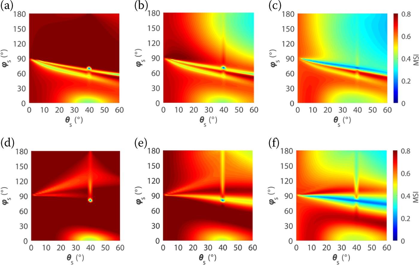
**FIGURE 5.13** MSI of RMS height derived from VV-polarized (top row: (**a–c**)) and HH-polarized (bottom row: (**d–f**)) scattering coefficients as a function of scattering angle ϑ_s and azimuth angle ϕ_s at L-band for incident angles ϑ_i of 40° with different correlation functions from left to right, i.e., (**a, d**) exponential, (**b, e**) 1.5-power, and (**c, f**) Gaussian.

In what follows, we examine the difference between TSI and MSI (TSI-MSI) of RMSH derived from VV-polarized and HH-polarized scattering coefficients as a function of scattering angle θ_s and azimuth angle ϕ_s at L-band for incident angles θ_i of 40° with exponential, 1.5-power and Gaussian correlation functions, as shown in Figure 5.14. For VV polarization, as shown in Figure 5.14(a–c), we can see that the interaction effects are generally small and close to zero for most parts of the whole upper half-space. That is, in these scattering geometries, the first-order (MSI) and total-order (TSI) sensitivity indices are almost equal. The interaction effects of RMS height with other parameters for HH polarization are examined in Figure 5.14(d–f). In general, the difference between TSI and MSI is very small on the whole upper half-space at L-band. The interactions of RMS height with other parameters are the highest at the exponentially correlated surface [29].

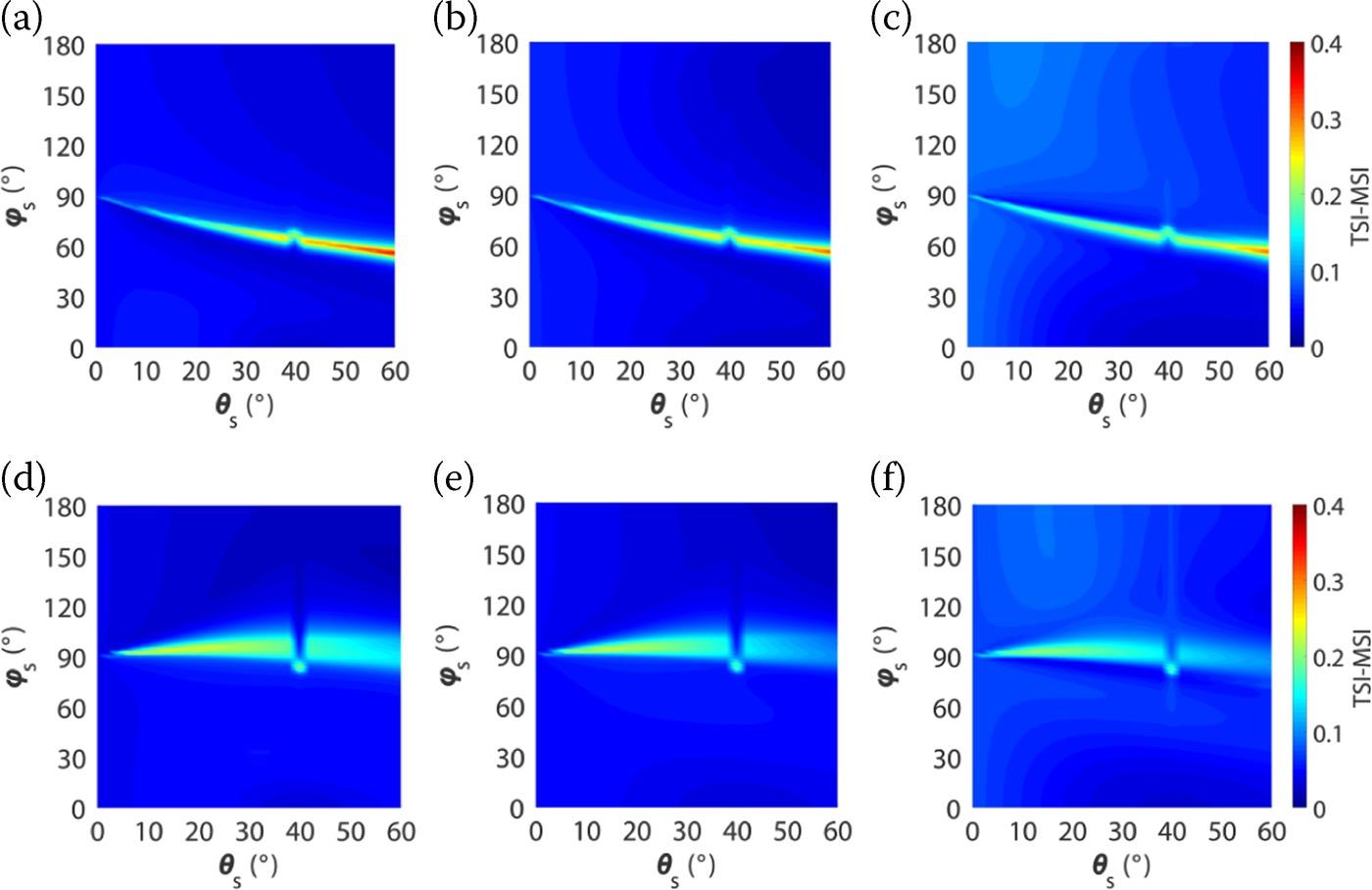
**FIGURE 5.14** TSI-MSI (the difference between TSI and MSI) of RMSH derived from VV-polarized (top row: (**a–c**)) and HH-polarized (bottom row: (**d–f**)) scattering coefficients as a function of scattering angle θ_s and azimuth angle ϕ_s at L-band for incident angles θ_i of 40° with different correlation functions from left to right, i.e., (**a, d**) exponential, (**b, e**) 1.5-power, and (**c, f**) Gaussian.

5.5.3 SENSITIVITY TO CORRELATION LENGTH

Figure 5.15 displays the MSI of correlation length that is associated with VV-polarized and HH-polarized bistatic scattering coefficients on the whole upper half-space as a function of scattering angle θ_s and azimuth angle ϕ_s for incident angles θ_i of 40° with exponential, 1.5-power and Gaussian correlation functions, respectively. For VV polarization, as shown in Figure 5.15(a–c), the sensitive zones of soil moisture are the largest for exponentially correlated surfaces and smallest for Gaussian-correlated surfaces. This is attributed to the significantly increased sensitivity of correlation length when the Gaussian correlation function is applied, implying that the sensitivity index of correlation length is much higher with the Gaussian correlation function than exponential correlation function for backscattering [29]. In contrast to soil moisture, the MSI distributions of the correlation length strongly depend on the correlation function. We can see that the sensitivities of correlation length are generally complementary, that is, the bistatic scattering coefficients show the lowest sensitivity to correlation length under exponential correlation function. The sensitivity of radar signals to correlation length increases significantly for the Gaussian correlation function. Compared with an exponential surface, a Gaussian surface is much more sensitive to the correlation length. Moreover, the sensitivity of correlation length near the specular region (i.e., θ_I = θ_s) always increases. This indicates that the specular region or quasi-specular region may be not preferred for soil moisture estimation due to the influence of the correlation length. In Figure 5.15(d–f), we investigate the distributions of MSI of the correlation length for HH-polarized scattering coefficients on the whole upper half-space as functions of scattering angle θ_s and azimuth angle ϕ_s for three incident angles and correlation functions. The sensitivity of correlation length is generally enhanced, regardless of the incident angles and correlation functions. In addition, the bistatic scattering shows the highest sensitivity to correlation length under the Gaussian correlation function for both HH and VV polarizations. This is because the Gaussian-correlated surface is more sensitive to correlation length, as already shown.

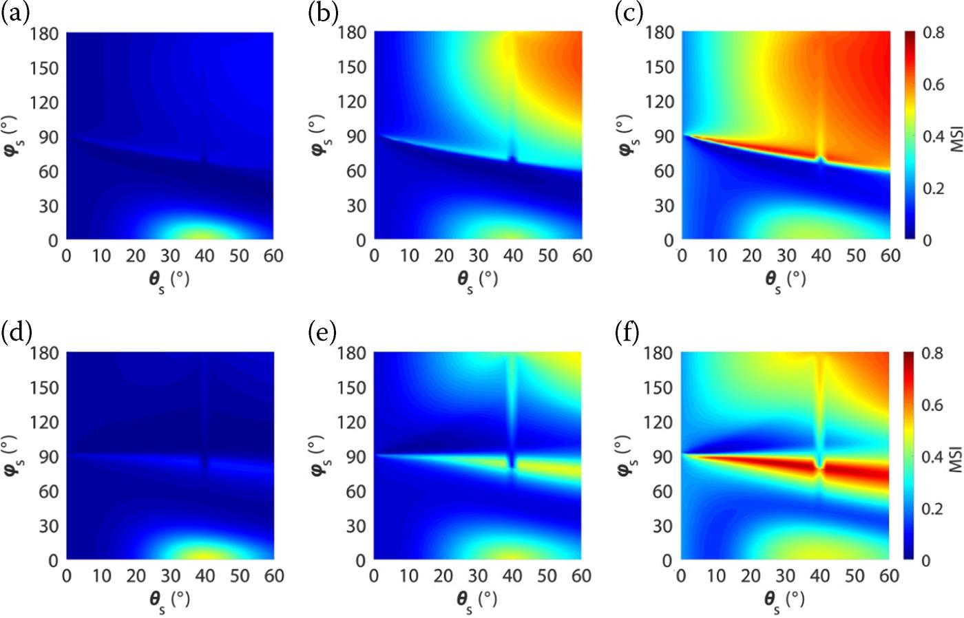
**FIGURE 5.15** MSI of the correlation length derived from VV-polarized (top row: (**a–c**)) and HH-polarized (bottom row: (**d–f**)) scattering coefficients as a function of scattering angle θ_s and azimuth angle ϕ_s at L-band for incident angles θ_i of 40° with different correlation functions from left to right, i.e., (**a, d**) exponential, (**b, e**) 1.5-power, and (**c, f**) Gaussian.

In Figure 5.16, we examine the difference between TSI and MSI (TSI-MSI) of correlation length derived from VV-polarized and HH-polarized scattering coefficients as a function of scattering angle θ_s and azimuth angle ϕ_s at L-band for incident angles θ_i of 40° with exponential, 1.5-power and Gaussian correlation functions, respectively. Note that the interaction effects are generally small and close to zero for most parts of the whole upper half-space. Figure 5.16(a–c) displays the interactions of correlation length with other parameters (e.g., soil moisture with RMS height, soil moisture with correlation length, and soil moisture with RMS height and correlation length). We see that the maximum interaction effects are very close to the cross-plane. Next, we investigate the interaction effects of correlation length with other parameters for HH polarization, as shown in Figure 5.16(d–f). In general, the difference between TSI and MSI for correlation length is very small on the whole upper half-space at L-band. In addition, we see that the distributions of interactions of soil moisture and RMS height are very similar, and the interaction effects of these two parameters are generally higher than those of correlation length, which is consistent with the results that were obtained for VV polarization. The interactions of correlation length with other parameters are the highest at the Gaussian-correlated surface.

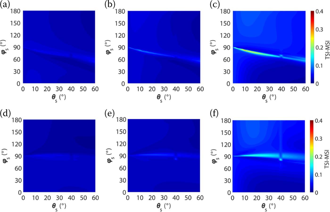
**FIGURE 5.16** TSI-MSI (the difference between TSI and MSI) of the correlation length derived from VV-polarized (top row: (**a–c**)) and HH-polarized (bottom row: (**d–f**)) scattering coefficients as a function of scattering angle ϑ_s and azimuth angle ϕ_s at L-band for incident angles ϑ_i of 40° with different correlation functions from left to right, i.e., (**a, d**) exponential, (**b, e**) 1.5-power, and (**c, f**) Gaussian.

At this point, we may draw a short summary regarding the parameter sensitivity conducted for the rough surface. Extensive analysis [29] show the SIs (TSI, MSI, and their difference) of soil moisture and surface roughness vary significantly for different bistatic configurations. In bistatic scattering, VV polarization is generally more sensitive to soil moisture than HH polarization, and the sensitivity becomes more remarkable as the incident angle increases. Both VV- and HH-polarized bistatic scattering show the highest sensitivity to soil moisture near the orthogonal plane at a small incident angle (e.g., 20°), but with very low returned signals and undesirable interaction effects. For VV polarization, the sensitive zone of soil moisture increases significantly as the incident angle increases. Moreover, these sensitive zone shifts toward the forward direction with small azimuth scattering angles and large scattering angles (i.e., farther away from the cross-plane), particularly at large incident angles (e.g., 60°). The scattering signals are measurable and preserve rich information on soil moisture at these geometries, making them favorable configurations for soil moisture retrieval. For HH polarization, as the incident angle increases, the high-sensitivity zone of soil moisture gradually becomes closer to the backward direction with large azimuth scattering angles and large scattering angles. However, an intermediate incident angle (e.g., 40°) is recommended for retrieving soil moisture when using HH-polarized bistatic scattering because low sensitivity is exhibited at small (e.g., 20°) and large incident angles (e.g., 60°) and in the presence of interaction effects.

It has been pointed out [30] that great care must be taken to estimate the sensitive parameters, while to assign those less sensitive parameters to a constant value for calibrating and for simplifying the scattering model. A study in [30] suggests that the parameter ranges affect both the SIs and their relative importance. A wider range of a given parameter corresponds to a larger SIs of that parameter. Parameters with the same range of variance but span different intervals exhibit different degrees of sensitivity. Smaller soil moisture and roughness generally exhibit higher sensitivity.

A final call is that specific receiver sensitivity, dynamic range, antenna footprint tracking, and synchronization, among others, in the context of the complex bistatic radar system. To this end, efforts to validate the optimal bistatic radar configurations by conducting indoor and field experiments as well as using real satellite bistatic measurements (e.g., Cyclone Global Navigation Satellite System) deserves further study.

References

1. Ulaby, F. T., and Long, D. G., Microwave Radar and Radiometric Remote Sensing, University of Michigan Press: Ann Arbor, MI, 2014.

2. Crosson, W. L., Limaye, A. S., and Laymon, C. A., Parameter sensitivity of soil moisture retrievals from airborne L-band radiometer measurements in SMEX02. IEEE Trans. on Geosci. Remote Sens., 43, 1517–1528, 2005.

3. Du, Y., Ulaby, F. T., and Dobson, M. C., Sensitivity to soil moisture by active and passive microwave sensors. IEEE Trans. on Geosci. Remote Sens., 38, 105–114, 2000.

4. Zribi, M., and Dechambre, M., A new empirical model to retrieve soil moisture and roughness from C-band radar data. Remote Sens. Environ., 84, 42–52, 2003.

5. Verhoest, N. E., Lievens, H., Wagner, W., Álvarez-Mozos, J., Moran, M. S., and Mattia, F., On the soil roughness parameterization problem in soil moisture retrieval of bare surfaces from synthetic aperture radar. Sensors, 8, 4213–4248, 2008.

6. Lievens, H., Verhoest, N. E., De Keyser, E., Vernieuwe, H., Matgen, P., Álvarez-Mozos, J., and De Baets, B., Effective roughness modeling as a tool for soil moisture retrieval from C-and L-band SAR. Hydrolol. Earth Sys., 15, 151–162, 2011.

7. Zribi, M., Gorrab, A., and Baghdadi, N., A new soil roughness parameter for the modelling of radar backscattering over bare soil, Remote Sens. Environ., 152, 62–73, 2014.

8. Pianosi, F., Sarrazin, F., and Wagener, T., A Matlab toolbox for global sensitivity analysis, Environ. Modeling Softw., 70, 80–85, 2015.

9. Saltelli, A., Ratto, M., and Andres, T., Global Sensitivity Analysis: The Primer, Chichester, Wiley, London, UK, 2008.

10. Saltelli, A., and Annoni, P., How to avoid a perfunctory sensitivity analysis, Environ. Modelling and Software, 25((12)), 1508–1517, 2010.

11. Saltelli, A., Tarantola, S., and Chan, K. S., A quantitative model-independent method for global sensitivity analysis of model output, Technometrics, 41((1)), 39–56, 1999.

12. Wang, J., Li, X., Lu, L., and Fang, F., Parameter sensitivity analysis of crop growth models based on the extended Fourier amplitude sensitivity test method. Environ. Model. and Softw., 48, 171–182, 2013.

13. Li, D., Jin, R., Zhou, J., and Kang, J., Analysis and reduction of the uncertainties in soil moisture estimation with the L-MEB model using EFAST and ensemble retrieval. IEEE Geosci. Remote Sens. Lett., 12, 1337–1341, 2015.

14. Lentini, N. E., and Hackett, E. E., Global sensitivity of parabolic equation radar wave propagation simulation to sea state and atmospheric refractivity structure. Radio Sci., 50, 1027–1049, 2015.

15. Neelam, M., and Mohanty, B. P., Global sensitivity analysis of the radiative transfer model. Water Resour. Res., 51, 2428–2443, 2015.

16. Petropoulos, G., and Srivastava, P. K., (Eds.), Sensitivity Analysis in Earth Observation Modelling, Elsevier, Oxford, UK, 2016.

17. Liu, H., Chen, W., and Sudjianto, A. Relative Entropy Based Method for Probabilistic Sensitivity Analysis in Engineering Design, Journal of Mechanical Design, 128((2)), 326. doi:10.1115/1.2159025, 2006.

18. Liu, Y., and Chen, K. S., An information entropy-based sensitivity analysis of radar sensing of rough surface. Remote Sensing, 10((2)), 286, 2018.

19. Sobol, I. M., Sensitivity estimates for nonlinear mathematical models, Math. Model. Comput. Experim., 1 (4), 407–414, 1993.

20. Cook, C. E., and Bernfeld, M., Radar Signals: An Introduction to Theory and Application, Artech House, Norwood, MA, 1993.

21. Lee, J. S., and Pottier, E., Polarimetric Radar Imaging: From Basics to Applications. CRC Press, Boca Raton, FL, 2009.

22. Cover, T. M., and Thomas, A., Elements of Information Theory, 2nd edn Edition, Wiley, New York, 2006.

23. Silverman, B. W., Density Estimation for Statistics and Data Analysis, Chapman and Hall/CRC Press, Boca Raton, FL, 1998.

24. Neelam, M., and Mohanty, B. P., Global sensitivity analysis of the radiative transfer model, Water Resour. Res., 51((4)), 2428–2443, 2015.

25. Zeng, J. Y., Chen, K. S., Bi, H. Y., Chen, Q., and Yang, X. F., Radar response of off-specular bistatic scattering to soil moisture and surface roughness at L-band, IEEE Geosci. Remote Sens. Lett., 13((2)), 1945–1949, 2016.

26. Kim, Y., and van Zyl, J. J., A time-series approach to estimate soil moisture using polarimetric radar data, IEEE Trans. Geosci. Remote Sens., 47((8)), 2519–2527, 2009.

27. Arii, M., van Zyl, J. J., and Kim, Y., A general characterization for polarimetric scattering from vegetation canopies, IEEE Trans. Geosci. Remote Sensing, 48((9)), 3349–3357, 2010.

28. Pierdicca, N., Guerriero, L., Comite, D., Brogioni, M., and Paloscia, S., Bistatic radar with large baseline for bio-geophysical parameter retrieval, Proc. IEEE IGARSS, 125–128, 2017.

29. Zeng, J. Y., Chen, K. S., Theoretical Study of Global Sensitivity Analysis of L-Band Radar Bistatic Scattering for Soil Moisture Retrieval, IEEE Geosci. Remote Sens. Letters, 15((11)), 1710–1714, 2018.

30. Ma, C., Li, X., and Wang, S., A global sensitivity analysis of soil parameters associated with backscattering using the advanced integral equation model, IEEE Trans. Geosci. Remote Sens., 53((10)), 5613–5623, 2015.

Tags: Radar Scattering and Imaging of Rough Surfaces Modeling and Applications with MATLAB

Jul 18, 2021 | Posted by admin in General Engineer | Comments Off

Engineer Key

Fastest Engineer Engine

Sensitivity Analysis of Radar Scattering of Rough Surface