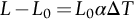
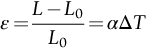
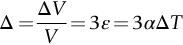
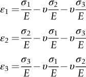
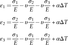
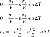
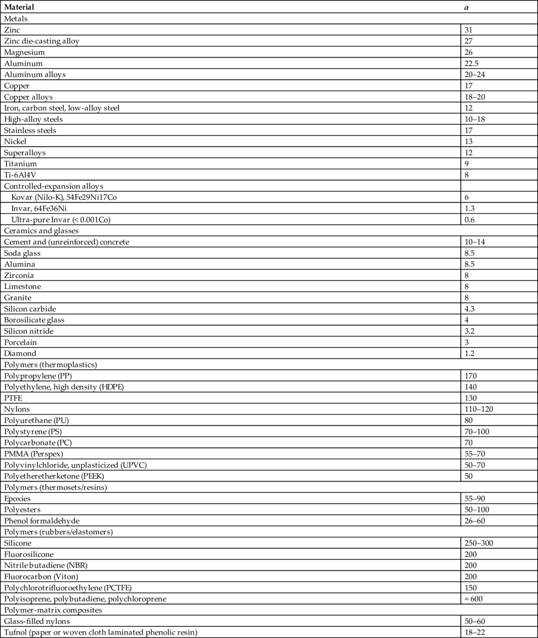
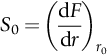
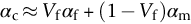
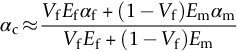
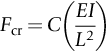
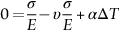
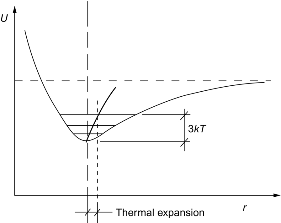
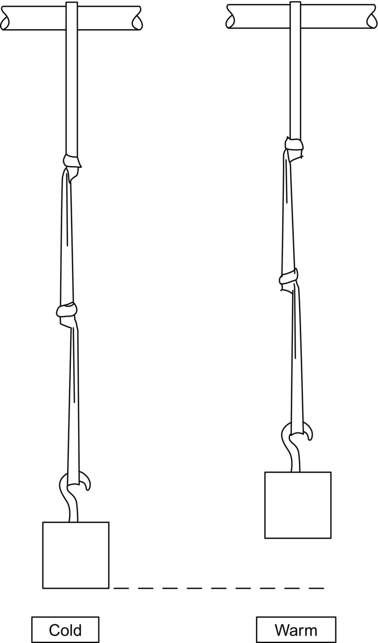
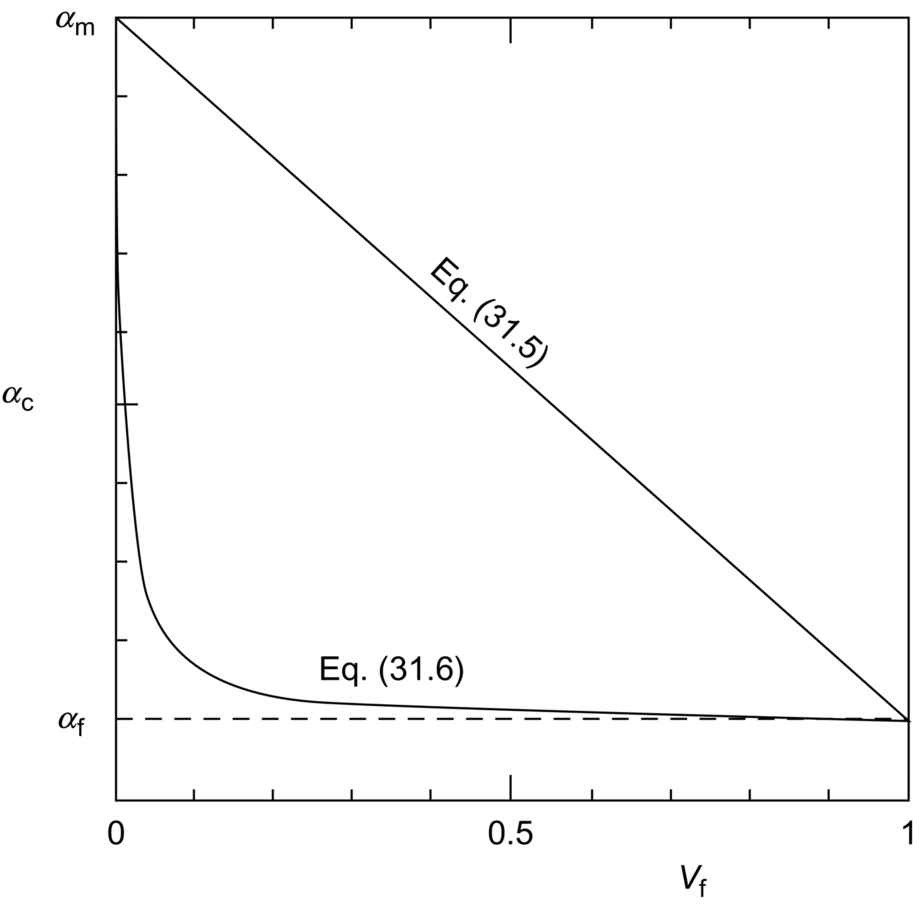
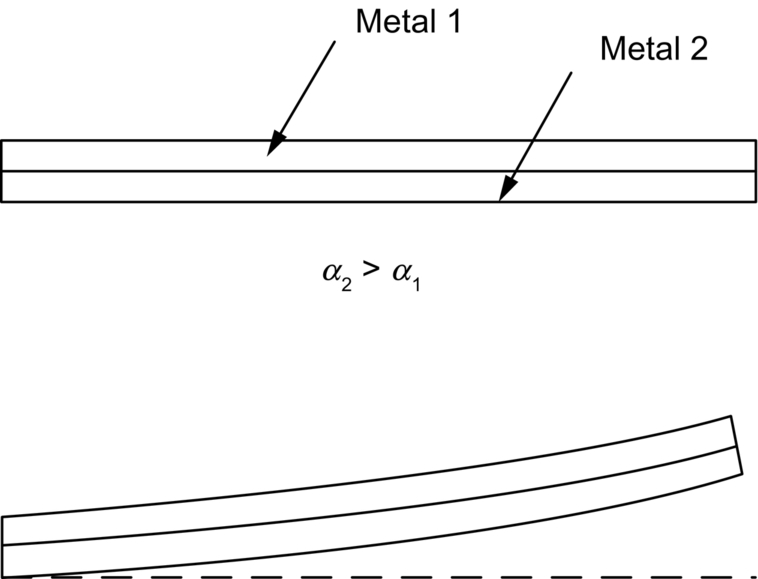
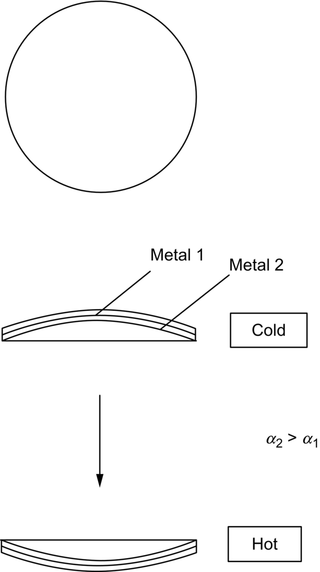
section epub:type=”chapter”> When solid materials are heated, most expand (although some very flexible rubbers actually contract). This expansion is defined by the linear coefficient of thermal expansion, α. If a rod-shaped specimen (having initial and final lengths L0 and L) is heated through a temperature interval ΔT, then This equation can be rewritten as. where ɛ is the (linear) thermal strain. For an isotropic material, the volume strain is given by We have already come across thermal expansion in several places: Section 17.4 (thermal cracking of PUR foam insulation panels); Chapter 18, Worked Example 1 (thermal fatigue of copper water-cooling plates); Example 18.7 (thermal fatigue in a boiler); Section 19.5 (residual stresses in welds); Example 29.11 (shrink fitting of compressor wheels). α is an important material property, with a huge range of applications—and consequences. In Section 17.4, we said that the thermal stress σ in the PUR foam was where E is Young’s modulus and υ is Poisson’s ratio. But how do we prove this? We saw in Example 7.11 that the elastic stress-strain relations for an isotropic material are We can easily modify these relations to include the effect of thermal expansion by simply adding the thermal strain to each strain component, giving Now let’s look at the free surface of the foam (see Figure 17.7). We locate principal axes 1p and 2p in the plane of the surface, and 3p perpendicular to the surface. σ3 = 0 (a free surface cannot support a stress) and ɛ1 = ɛ2 = 0 (the surface cannot contract sideways, because it is fixed to the steel plate). So This gives σ1 = σ2 = σ (equibiaxial), (Note that ΔT is negative, because the free surface of the foam has been cooled. So σ is a tensile stress.)■ How do we measure α? As a rough approximation for many metals and ceramics, a temperature rise of 100°C produces a thermal strain of one in a thousand (equivalent to 1 thou per inch). Measuring α for these materials therefore requires very accurate measurement of length and precise control of temperature. This presents considerable challenges, especially when measurements have to be done at high temperatures. If traditional mechanical methods (e.g., micrometers, displacement transducers) are used, great care must be taken that the measuring equipment itself does not expand (or if it does, this is calibrated out). Most of these problems have now been solved using noncontact methods, such as laser interferometry (which is also extremely accurate). Data for α are shown in Table 31.1. Within each materials class the values vary a lot, although the range of values for metals and ceramics is much the same. What is notable, however, are the large values for polymers (and some polymer-based composites)—typically 5 or 10 times those for metals and ceramics. α itself is a weak function of temperature—the values shown in the table are average values over a finite temperature range (often 25–125°C). For exacting applications, data must be obtained over the relevant temperature range, which may be hundreds of degrees higher. But what causes the positive thermal expansion of most materials, and the large differences between metals/ceramics and polymers/composites? In Chapter 4, we looked at the physics of bonding between atoms, in order to explain the origin of Young’s modulus. It turns out that interatomic bonding is also key to understanding the origin of thermal expansion. Figure 31.1 is a version of Figure 4.6, showing the net energy/distance U(r) curve for a bond. Now we saw in Chapter 22 (Section 22.2) that the atoms in a solid vibrate (or oscillate) about their mean positions. At a given absolute temperature T, the thermal energy of a vibrating atom is 3kT averaged over time (k = Boltzmann’s constant). Figure 31.1 shows the average thermal energy of the atom drawn as a horizontal line, sitting above the minimum of the “potential well.” The length of this line, between the sides of the potential well, represents the average amplitude of vibration of the atoms. As the temperature T is increased, the thermal energy of the atoms 3kT increases in proportion, and the vibrational energy level moves upwards within the potential well. The amplitude of vibration of the atoms also increases (the line has got a bit longer). But what is really interesting is that the center of vibration of the atoms has moved outwards—the atoms in the solid have all moved away from one another, and this produces thermal expansion. This is all a consequence of the asymmetry of the U(r) curve, which in turn is down to the fact that the repulsion term in the interatomic potential is generally much steeper than the attraction term (see Equation (4.4)). But why, for example, is α only 1.2 × 10− 6 K− 1 for diamond, when it is 22.5 × 10− 6 K− 1 for aluminum? This is explained by the U(r) curves: the potential well for aluminum is wider and shallower than for diamond. This is the consequence of the different interatomic bonding in these two materials—covalent in diamond, metallic in aluminum. As you can see from Figure 4.11, a narrow potential well (small rD − r0) gives a large slope dF/dr at the equilibrium separation r0, and a wide potential well (large rD − r0) gives a small dF/dr at r0. We know that the bond stiffness (see Equations (4.7) and (4.8)), and we know that Young’s modulus E = S0/r0 (see Equation (6.5)), so we would expect the thermal expansion of any material to be correlated with its Young’s modulus. This is broadly true: E for diamond (1000 GN m− 2) is approximately 15 times larger than E for aluminum (69 GN m− 2); and α for diamond is approximately 19 times smaller than α for aluminum. In fact, for a wide range of materials (including many polymers), where C is a constant. ■ Looking now at polymers (see Table 31.1), α goes from 26 × 10− 6 K− 1 for thermosets, to 170 × 10− 6 K− 1 for thermoplastics above the glass temperature TG. This, again, reflects the nature of the bonding (see Figures 5.10 and 6.2): in thermosets, there are lots of stiff, covalent crosslinks; in thermoplastics above TG, there are much weaker constraints (crystalline regions and occasional branches/tangles, but no Van der Waals bonds). Rubbers are interesting. As shown in Table 31.1, α for rubbers goes from 150 × 10− 6 K− 1 for PCTFE, to around 600 × 10− 6 K− 1 for polyisoprene. The polymer chains are held together by occasional covalent crosslinks (see Figures 5.10(a)), but the chain segments between these crosslinks are able to move in response to stress. If the rubber is loaded, the chain segments straighten out a bit, and the rubber extends. The chain segments become more ordered as they straighten out, and work is required to produce this ordering. This chain straightening is the origin of the low Young’s modulus of rubbers (see Figure 6.2). This low stiffness should correlate with a large value of α, and in fact it does. However, some (very flexible) rubbers have a negative α—they contract when heated. You can easily show this at home (see Figure 31.2). Tie a few large rubber bands together end to end to form one long length of rubber. Hang one end from a convenient support, and put a small weight on the other end. Then warm the rubber up with a hair dryer. Keep the drier moving slowly up and down the length of rubber so as not to overheat any part of it. You will see the weight move up by several cm as the rubber warms up and contracts. Because there are so few crosslinks in soft rubber, the chain segments are very long. When the atoms in the segments vibrate, the segments actually bow out sideways, and this pulls the ends of the segments toward one another. If we look at the composite geometry shown in Figure 6.3(b), we can see that the overall expansion coefficient perpendicular to the fibers should be given by the weighted average of the individual expansion coefficients. The overall expansion coefficient parallel to the fibers (Figure 6.3(a)) is given by We won’t derive this result here, but the terms in Young’s modulus appear because the difference in thermal expansion between fibers and matrix must be neutralized with opposing elastic deflections (and hence forces) in fibers and matrix. (If any reader would like a challenge, they can verify Equation (31.6) using the condition that the net internal force parallel to the fibers must be zero.) We have plotted Equations (31.5) and (31.6) in Figure 31.3. The line for Equation (31.6) uses values of αm = 10αf and Ef = 100Em. αc values for particulate composites lie between these two lines. Looking at Table 31.1, we can see that α for nylon is 110–120 × 10− 6 K− 1, whereas α for glass-filled nylon is only 50–60 × 10− 6 K− 1. This reduction in α is what Equations (31.5) and (31.6) predict. In many applications, polymers are filled just to reduce thermal expansion. Tufnol, too, has a value of α (18–22 × 10− 6 K− 1), which is around half that of unreinforced (phenolic) resin (26–60 × 10− 6 K− 1). Things like electric toasters and kettles use bimetals to cut off the electricity to the heating element when a preset temperature is reached. Two metals with different values of α are joined together in the form of a thin beam (Figure 31.4). When the temperature increases, the beam bends. We have already seen what happens when you bend a beam into a radius R (see Figure 7.1). The inside of the curve gets a little shorter, and the outside gets a little longer. In a bimetal beam, since one side of the bimetal beam expands more than the other side, the beam must bend into a radius R to relieve the thermal stresses. This movement is used to actuate an electrical switch. A very clever type of bimetal is the “snap-through disc.” This is made slightly domed at room temperature (see Figure 31.6). As the temperature increases, the shape of the disc remains the same, but the differential expansion of the two metals produces a locked-in thermal stress. Eventually, the domed disc can no longer support the thermal stress, and it “snaps through” as shown in Figure 31.5. The advantages of this type of bimetal are (a) it can be finely tuned to trip at a particular temperature, (b) it delivers enough movement and force to fully open a switch in an instant (this avoids arcing). When the bimetal cools down again, the thermal stress builds up in the reverse direction, until the disc snaps back to its original shape. When you next boil an electric kettle, listen for the disc tripping the power, then continue to listen very carefully once the water has stopped boiling. After a few minutes you will hear a quiet but definite “click.” This is the bimetal disc snapping back to its original shape on the way back down. Traditional railroad track is hot rolled to the correct cross section in the steel mill, and cut into standard lengths for easy transportation. When the track is laid, the lengths are joined end to end using “fishplates”—short lengths of steel plate overlapping the joint, and bolted to the ends of the rails (Figure 31.6). At each joint there must be a short gap (≈ 1/8″) between the rail ends, to allow for longitudinal thermal expansion of the rails on hot days. Fishplate joints are unsatisfactory for high-speed lines, and these now use continuous welded rail (CWR). Rail from the mill is delivered to site by train in long prewelded lengths, laid on reinforced concrete ties (sleepers), and finally site welded into still longer lengths (many km long). Figure 31.7 is a close up of a section of rail showing the ties, and the spring clips that hold the rail down onto the ties. The rail is subjected to a range of temperatures, from the coldest temperatures in winter to the hottest days in summer. In continental US or Europe this can easily be − 10 to + 30°C (ΔT = 40°C), giving a thermal strain αΔT of 12 × 10− 6 × 40, or 0.48 × 10− 3 (α value of steel taken from Table 31.1). Over a 3-km length of CWR, this would produce a length change of 1.44 m! Clearly, something has to be done to stop the rail expanding/contracting. For each km of track, there will approximately 2000 ties, so there are 2000 clips bearing down on each rail. The combined friction of all these clips stops the rail sliding over the ties. The ties themselves are very heavy, and are set in tightly packed ballast consisting of self-locking chips of broken stone (e.g., granite). This means that the ties do not move over the ground either, so the track is unable to expand or contract. The thermal strain is neutralized by an equal and opposite elastic strain, which produces a locked-in thermal stress given by For ΔT = 40°C, σ = 200 × 103 MN m− 2 × 0.48 × 10− 3 = 96 MN m− 2 (E value of ferritic steel taken from Table 3.1). This is much less than the yield stress of the steel, so the rail stays elastic. There is one complication, though. On very hot days, the compression force in the rail can cause buckling—the track moves sideways, and tight snaking curves develop which will derail a train. We have already looked at the elastic buckling of beams in Chapter 7. The critical buckling load is given by Modern rail sections have a large second moment of area I, so this helps to stop buckling. However, the rail is very long (large L), so if the rail is not prevented from moving sideways, it will buckle very easily. In practice, the heavy ties and strong ballast generally stop the rail moving sideways as well as lengthways, and the risk of buckling is small. However, in practice, this risk is further reduced by ensuring that the rail spends a lot of its time in tension. After the rail is laid, but before it is site welded and clipped to the ties, it is pretensioned using powerful hydraulic jacks. Of course, after a long patch of warm weather—when the stock of rail has had time to warm up—this pretensioning may not be needed. The service temperature at which the rail neither expands nor contracts is called the “zero-stress temperature,” and this is generally chosen so as to engineer a low risk of buckling at the maximum design temperature, while ensuring that the rail does not pull through the spring clips at the minimum design temperature. In Figure 26.5, we looked at an example of a glass-to-metal seal between the casing of a device and a wire conductor, designed to insulate the casing from the conductor. Both the casing and the wire were made from Kovar—a controlled expansion alloy (α = 6 × 10− 6 K− 1, see Table 31.1). Small beads of low-expansion borosilicate glass (α = 4 × 10− 6 K− 1, see Table 31.1) were placed between the casing and the conductor, and when the vacuum furnace came up to temperature (1000°C) the glass flowed and wetted the oxide-free metal surfaces. The power to the furnace was then switched off, and the assembly allowed to cool to room temperature. On cooling from 1000 to 20°C, the casing, glass, and conductor all contract by αΔT. The α values for Kovar and borosilicate glass are small, and very similar, so the thermal stresses in the seal at room temperature will be small. This is particularly important in the case of glass—a brittle material, which cracks easily in response to tensile thermal stress.
Thermal Expansion
31.1 Introduction
Worked Example 1
 , and
, and  .
.
31.2 Coefficients of Thermal Expansion
31.3 Physical Basis of Thermal Expansion
Worked Example 2
31.4 Thermal Expansion of Composites
31.5 Case Studies
Temperature switches
Continuous welded railroad track


Glass-to-metal seals
Examples
Answers