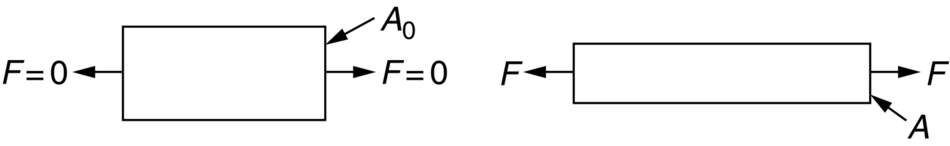
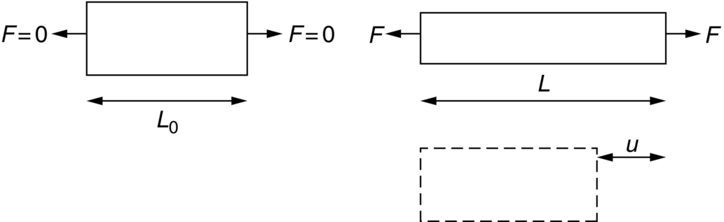
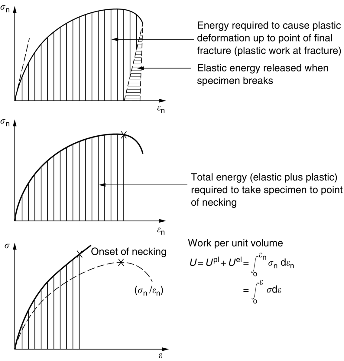
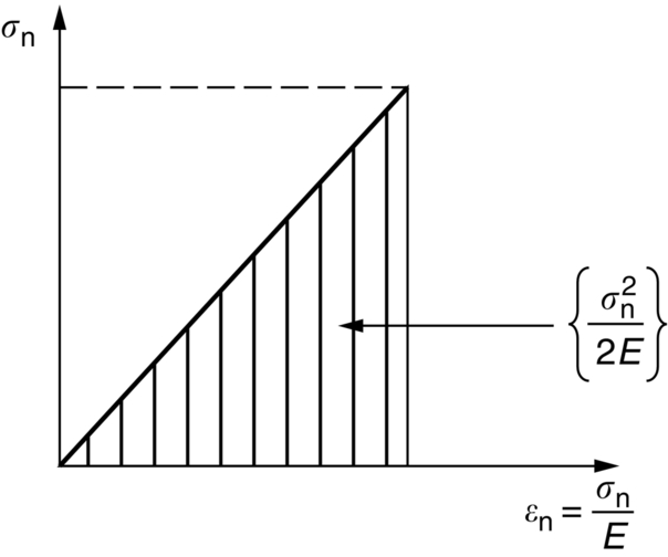
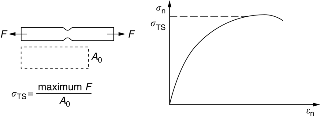
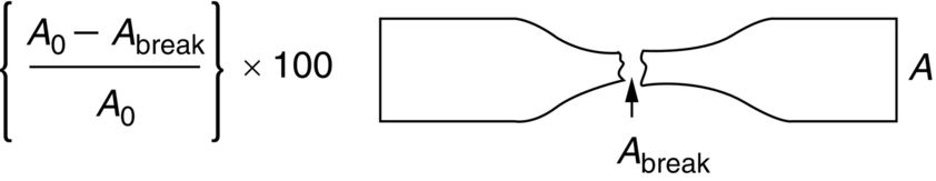
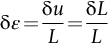
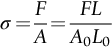
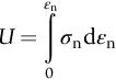
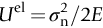
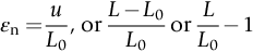
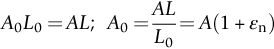
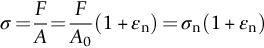
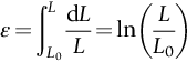
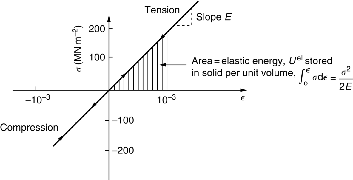
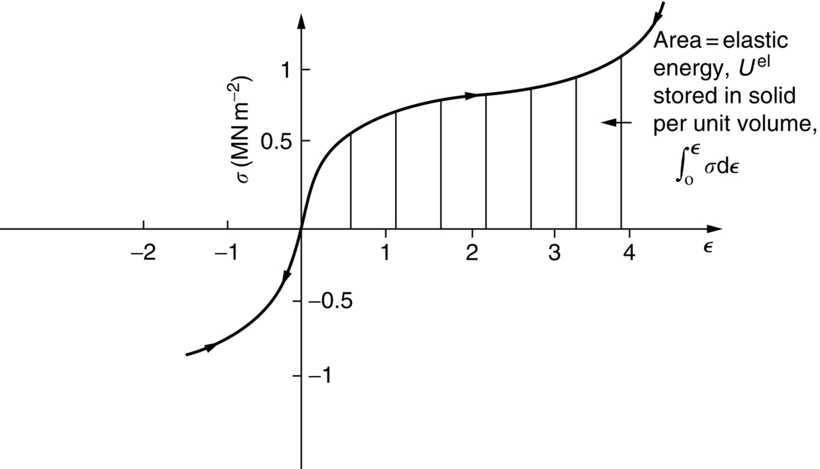
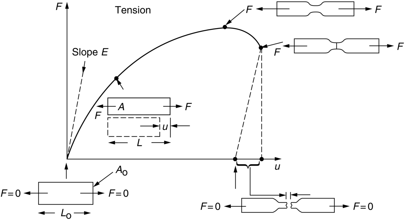
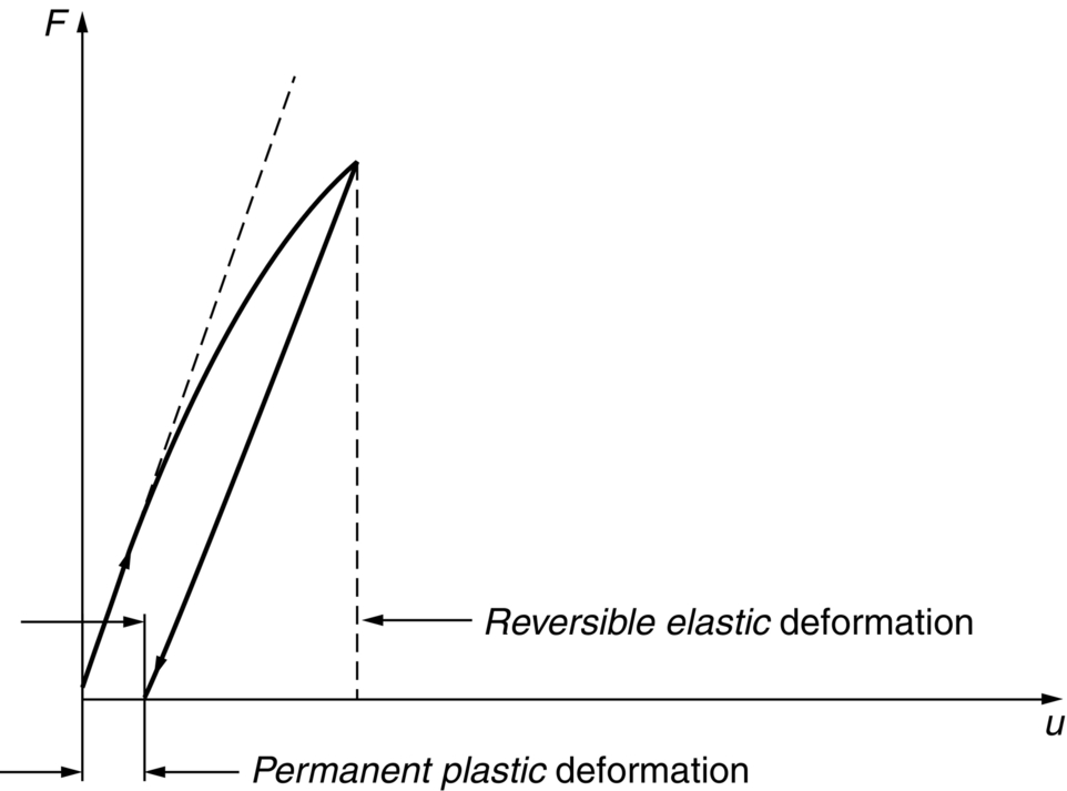
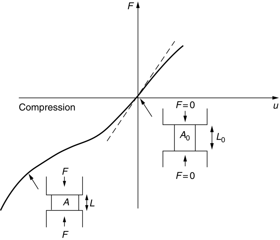
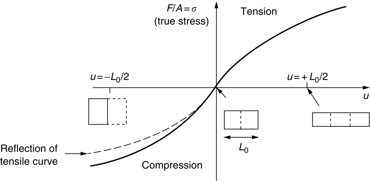
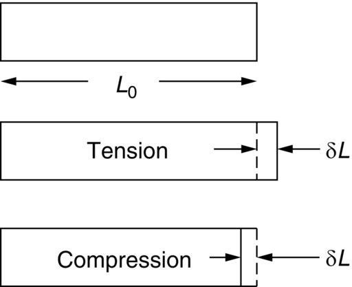
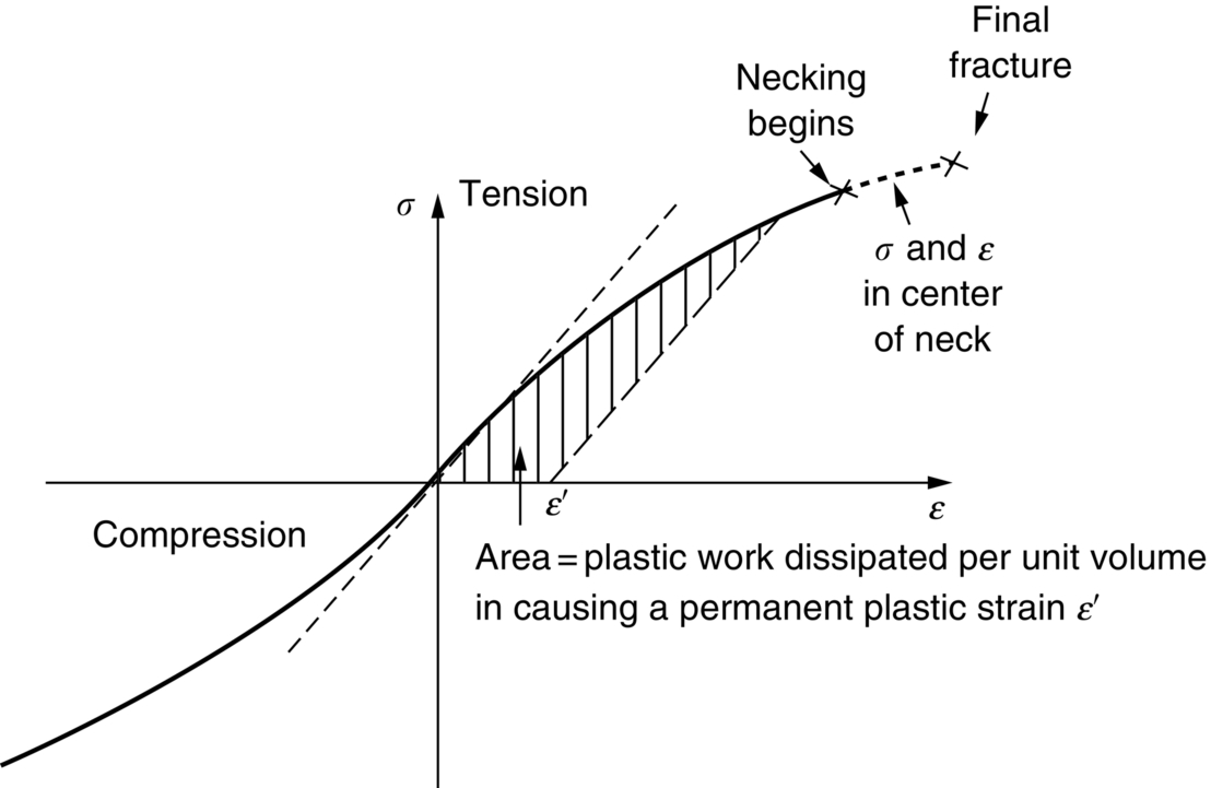
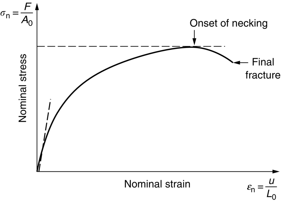
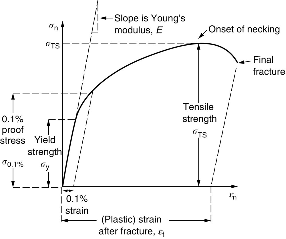
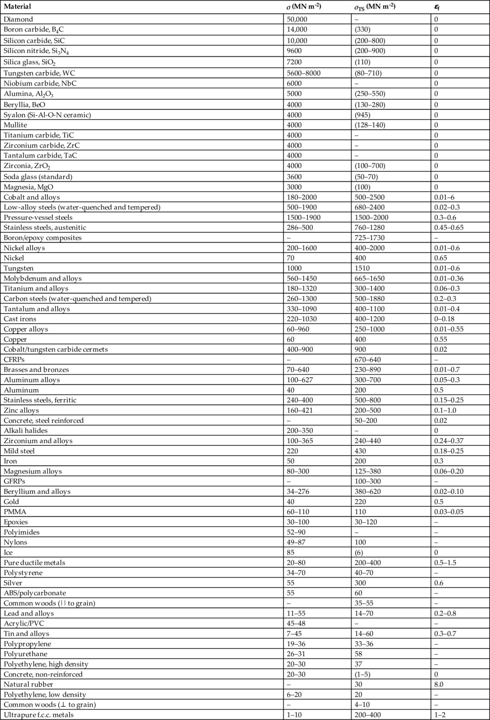
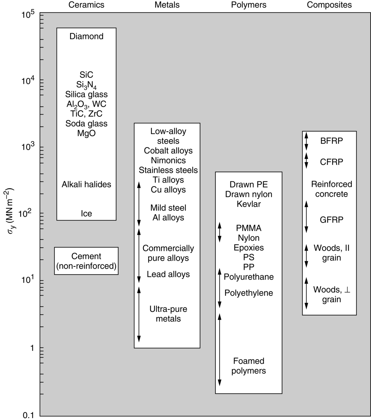
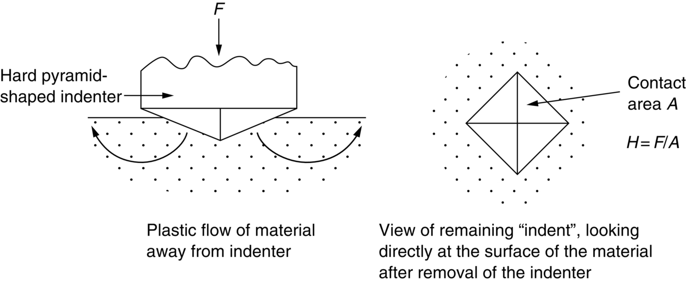
section epub:type=”chapter”> All solids have an elastic limit beyond which something happens. A totally brittle solid may fracture suddenly (e.g., glass). Most engineering materials do something different; they deform plastically or change their shapes in a permanent way. It is important to know when, and how, they do this—to design structures to withstand normal service loads without any permanent deformation, and rolling mills, sheet presses and forging machinery that will be strong enough to deform the materials that are formed. To study this, prepared samples are carefully pulled in a tensile testing machine, or they are compressed in a compression machine, and the stress required to produce a given strain is recorded. This chapter starts with a discussion on linear and nonlinear elasticity. Rubbers are exceptional in behaving elastically to high strains; almost all materials, when strained by more than about 0.001 (0.1%), do something irreversible: and most engineering materials deform plastically to change their shape permanently. This section discusses load–extension curves for nonelastic (plastic) behavior, followed by a discussion on true stress–strain curves for plastic flow. Next this chapter focuses on plastic work and tensile testing. This is followed by the discussion on data for yield strength, tensile strength, and tensile ductility. This chapter concludes with a note on the hardness test. All solids have an elastic limit beyond which something happens. A totally brittle solid will fracture suddenly (e.g., glass). Most engineering materials do something different; they deform plastically or change their shapes in a permanent way. It is important to know when, and how, they do this—so we can design structures to withstand normal service loads without any permanent deformation; and rolling mills, presses and forging machinery strong enough to deform the materials being rolled, pressed or forged. To study this, we pull carefully prepared samples in a tensile testing machine, or compress them in a compression machine, and record the stress required to produce a given strain. Figure 9.1 shows the stress–strain curve of a material exhibiting perfectly linear elastic behavior. This is the behavior that is characterized by Hooke’s law (Chapter 3). All solids are linear elastic at small strains—by which we usually mean less than 0.001, or 0.1%. The slope of the stress–strain line, which is the same in compression as in tension, is Young’s modulus, E. The area (shaded) is the elastic energy stored, per unit volume: we can get it all back if we unload the solid, which behaves like a spring. Figure 9.2 shows a nonlinear elastic solid. Rubbers have a stress–strain curve like this, extending to very large strains (of order 5 or even 8). The material is still elastic: if unloaded much of the energy stored during loading is recovered—that is why catapults can be as lethal as they are. Rubbers are exceptional in behaving elastically to high strains; as we said, almost all materials, when strained by more than about 0.001 (0.1%), do something irreversible: and most engineering materials deform plastically to change their shape permanently. If we load a piece of ductile metal (e.g., copper), in tension, we get the following relationship between the load and the extension (Figure 9.3). This can be demonstrated nicely by pulling a piece of plasticine modelling clay (a ductile non-metallic material). Initially, the plasticine deforms elastically, but at a small strain begins to deform plastically, so if the load is removed, the piece of plasticine is permanently longer than it was at the beginning of the test: it has undergone plastic deformation (Figure 9.4). If you continue to pull, it continues to get longer, at the same time getting thinner because in plastic deformation volume is conserved (matter is just flowing from place to place). Eventually, the plasticine becomes unstable and begins to neck at the maximum load point in the force-extension curve (see Figure 9.3). Necking is an instability which we shall look at in more detail in Chapter 12. The neck grows rapidly, and the load that the specimen can carry through the neck decreases until breakage takes place. The two pieces produced after breakage have a total length that is slightly less than the length just before breakage by the amount of the elastic extension produced by the terminal load. If we load a material in compression, the force-displacement curve is simply the reverse of that for tension at small strains, but it becomes different at larger strains. As the specimen squashes down, becoming shorter and fatter to conserve volume, the load needed to keep it flowing rises (Figure 9.5). No instability such as necking appears, and the specimen can be squashed almost indefinitely, only being limited by severe cracking in the specimen or plastic flow of the compression plates. The apparent difference between the curves for tension and compression is due solely to the geometry of testing. If, instead of plotting load, we plot load divided by the actual cross-sectional area of the specimen, A, at any particular elongation or compression, the two curves become much more like one another. In other words, we simply plot true stress (see Chapter 3) as our vertical coordinate (Figure 9.6). This method of plotting allows for the thinning of the material when pulled in tension, or the fattening of the material when compressed. Figure 9.6 But the two curves still do not exactly match, as Figure 9.6 shows. The reason is that a displacement of (for example) u = L0/2 in tension and in compression gives different strains; it represents a drawing out of the tensile specimen from L0 to 1.5L0, but a squashing down of the compressive specimen from L0 to 0.5L0. The material of the compressive specimen has thus undergone much more plastic deformation than the material in the tensile specimen, and can hardly be expected to be in the same state, or to show the same resistance to plastic deformation. The two conditions can be compared properly by taking small strain increments about which the state of the material is the same for either tension or compression (Figure 9.7). Figure 9.7 This is the same as saying that a decrease in length from 100 mm (L0) to 99 mm (L), or an increase in length from 100 mm (L0) to 101 mm (L) both represent a 1% change in the state of the material. Actually, they do not give exactly the same state in both cases, but they do in the limit Then, if the stresses in compression and tension are plotted against the two curves exactly mirror one another (Figure 9.8). The quantity ɛ is called the true strain (to be contrasted with the nominal strain u/L0 defined in Chapter 3) and the matching curves are true stress/true strain (σ/ɛ) curves. Figure 9.8 Now, a final catch. From our original load-extension or load-compression curves we can easily calculate ɛ, simply by knowing L0 and taking natural logs. But how do we calculate σ? Because volume is conserved during plastic deformation we can write, at any strain, provided the extent of plastic deformation is much greater than the extent of elastic deformation (volume is only conserved during elastic deformation if Poisson’s ratio v = 0.5; and it is near 0.33 for most materials). Thus and all of which we know or can measure easily. When metals are rolled or forged, or drawn to wire, or when polymers are injection molded or pressed or drawn, energy is absorbed. The work done on a material to change its shape permanently is called the plastic work; its value, per unit volume, is the area of the crosshatched region shown in Figure 9.8; it may easily be found (if the stress–strain curve is known) for any amount of permanent plastic deformation, ɛ′. Plastic work is important in metal and polymer forming operations because it determines the forces that the rolls, or press or molding machine must exert on the material. The plastic behavior of a material is usually measured by conducting a tensile test. Tensile testing equipment is standard in engineering laboratories. Such equipment produces a load/displacement (F/u) curve for the material, which is then converted to a nominal stress/nominal strain, or σn/ɛn, curve (see Figure 9.9), where and Figure 9.9 Naturally, because A0 and L0 are constant, the shape of the σn/ɛn curve is identical to that of the load-extension curve. But the σn/ɛn plotting method allows us to compare data for specimens having different (though now standardized) A0 and L0, and thus to examine the properties of material, unaffected by specimen size. The advantage of keeping the stress in nominal units and not converting to true stress (as shown before) is that the onset of necking can clearly be seen on the σn/ɛn curve. Now, we define the quantities usually listed as the results of a tensile test. The easiest way to do this is to show them on the σn/ɛn curve itself (Figure 9.10). They are: Figure 9.10 Data for yield strength, tensile strength, and tensile ductility are given in Table 9.1 and shown on the bar chart (Figure 9.11). Like moduli, they span a range of about 106: from about 0.1 MN m-2 (for polystyrene foams) to nearly 105 MN m-2 (for diamond). Table 9.1 Note: Bracketed σTS data for brittle materials refer to the modulus of rupture σr (see Chapter 16). Most ceramics have enormous yield stresses. In a tensile test, at room temperature, ceramics almost all fracture long before they yield: this is because their fracture toughness, which we will discuss later, is very low. Because of this, you cannot measure the yield strength of a ceramic by using a tensile test. Instead, you have to use a test that somehow suppresses fracture: a compression test, for instance. The best and easiest is the hardness test. Pure metals are very soft indeed, and have a high ductility. This is what, for centuries, has made them so attractive at first for jewellery and weapons, and then for other implements and structures: they can be worked to the shape that you want them in; furthermore, their ability to work-harden means that, after you have finished, the metal is much stronger than when you started. By alloying, the strength of metals can be further increased, though—in yield strength—the strongest metals still fall short of most ceramics. Polymers, in general, have lower yield strengths than metals. The very strongest barely reach the strength of aluminum alloys. They can be strengthened, however, by making composites out of them: GFRP has a strength only slightly inferior to aluminum, and CFRP is substantially stronger. The hardness test is used for estimating the yield strengths of hard brittle materials. It is also widely used as a simple non-destructive test on material or finished components to check whether they meet the specified mechanical properties. Figure 9.12 shows how one type of test works (the diamond pyramid test). A very hard (diamond) pyramid “indenter” (with a standardized angle of 136° between opposite faces) is pressed into the surface of the material with a force F. Material flows away from underneath the indenter, so when the indenter is removed again, a permanent “indent” is left. The diagonals of the indent are measured with a microscope, and the total surface (or contact) area A of the indent is found from look-up tables. The hardness H is then given by H = F/A. Obviously, the softer the material, the larger the indents. The yield strength can be estimated from the relation (derived in Chapter 12) When flowing away from the indenter, the material experiences an average nominal strain of 0.08. This means that Equation (9.8) is only accurate for materials which do not work harden. For materials that do, the hardness test gives the yield strength of material that has been work hardened by 8%. Good correlations can also be obtained between hardness and tensile strength. For example, holds well (to ± 10%) for all types of steel. The indentation hardness is defined slightly differently—still as H = F/A, but A is now the area of the indent measured at the surface of the material (which is slightly less than that measured on the faces of the indentation). σn, nominal stress σn = F/A0 σ, true stress σ = F/A ɛn, nominal strain Relations between σn, σ and ɛn Assuming constant volume (valid if υ = 0.5 or, if not, plastic deformation ≫ elastic deformation): Thus ɛ, true strain and the relation between ɛ and ɛn Thus Small strain condition For small ɛn Thus, when dealing with most elastic strains (but not in rubbers), it is immaterial whether ɛ or ɛn, or σ or σn, are chosen. Energy The energy expended in deforming a material per unit volume is given by the area under the stress–strain curve. For linear elastic strains, and only linear elastic strains Elastic limit In a tensile test, as the load increases, the specimen at first is strained elastically, that is reversibly. Above a limiting stress—the elastic limit—some of the strain is permanent; this is plastic deformation. Strain hardening (work-hardening) The increase in stress needed to produce further strain in the plastic region. Each strain increment strengthens or hardens the material so that a larger stress is needed for further strain. σTS, tensile strength (ultimate tensile strength, or UTS) ɛf, strain after fracture, or tensile ductility The permanent extension in length (measured by fitting the broken pieces together) expressed as a percentage of the original gauge length. Reduction in area at break The maximum decrease in cross-sectional area at the fracture expressed as a percentage of the original cross-sectional area. Strain after fracture and percentage reduction in area are used a measures of ductility, that is the ability of a material to undergo large plastic strain under stress before it fractures.
Yield Strength, Tensile Strength, and Ductility
Publisher Summary
9.1 Introduction
9.2 Linear and Nonlinear Elasticity
9.3 Load–Extension Curves for Nonelastic (Plastic) Behavior
9.4 True Stress–Strain Curves for Plastic Flow
9.5 Plastic Work
9.6 Tensile Testing
9.7 Data
Material
σ (MN m-2)
σTS (MN m-2)
ɛf
Diamond
50,000
–
0
Boron carbide, B4C
14,000
(330)
0
Silicon carbide, SiC
10,000
(200–800)
0
Silicon nitride, Si3N4
9600
(200–900)
0
Silica glass, SiO2
7200
(110)
0
Tungsten carbide, WC
5600–8000
(80–710)
0
Niobium carbide, NbC
6000
–
0
Alumina, Al2O3
5000
(250–550)
0
Beryllia, BeO
4000
(130–280)
0
Syalon (Si-Al-O-N ceramic)
4000
(945)
0
Mullite
4000
(128–140)
0
Titanium carbide, TiC
4000
–
0
Zirconium carbide, ZrC
4000
–
0
Tantalum carbide, TaC
4000
–
0
Zirconia, ZrO2
4000
(100–700)
0
Soda glass (standard)
3600
(50–70)
0
Magnesia, MgO
3000
(100)
0
Cobalt and alloys
180–2000
500–2500
0.01–6
Low-alloy steels (water-quenched and tempered)
500–1900
680–2400
0.02–0.3
Pressure-vessel steels
1500–1900
1500–2000
0.3–0.6
Stainless steels, austenitic
286–500
760–1280
0.45–0.65
Boron/epoxy composites
–
725–1730
–
Nickel alloys
200–1600
400–2000
0.01–0.6
Nickel
70
400
0.65
Tungsten
1000
1510
0.01–0.6
Molybdenum and alloys
560–1450
665–1650
0.01–0.36
Titanium and alloys
180–1320
300–1400
0.06–0.3
Carbon steels (water-quenched and tempered)
260–1300
500–1880
0.2–0.3
Tantalum and alloys
330–1090
400–1100
0.01–0.4
Cast irons
220–1030
400–1200
0–0.18
Copper alloys
60–960
250–1000
0.01–0.55
Copper
60
400
0.55
Cobalt/tungsten carbide cermets
400–900
900
0.02
CFRPs
–
670–640
–
Brasses and bronzes
70–640
230–890
0.01–0.7
Aluminum alloys
100–627
300–700
0.05–0.3
Aluminum
40
200
0.5
Stainless steels, ferritic
240–400
500–800
0.15–0.25
Zinc alloys
160–421
200–500
0.1–1.0
Concrete, steel reinforced
–
50–200
0.02
Alkali halides
200–350
–
0
Zirconium and alloys
100–365
240–440
0.24–0.37
Mild steel
220
430
0.18–0.25
Iron
50
200
0.3
Magnesium alloys
80–300
125–380
0.06–0.20
GFRPs
–
100–300
–
Beryllium and alloys
34–276
380–620
0.02–0.10
Gold
40
220
0.5
PMMA
60–110
110
0.03–0.05
Epoxies
30–100
30–120
–
Polyimides
52–90
–
–
Nylons
49–87
100
–
Ice
85
(6)
0
Pure ductile metals
20–80
200–400
0.5–1.5
Polystyrene
34–70
40–70
–
Silver
55
300
0.6
ABS/polycarbonate
55
60
–
Common woods (|| to grain)
–
35–55
–
Lead and alloys
11–55
14–70
0.2–0.8
Acrylic/PVC
45–48
–
–
Tin and alloys
7–45
14–60
0.3–0.7
Polypropylene
19–36
33–36
–
Polyurethane
26–31
58
–
Polyethylene, high density
20–30
37
–
Concrete, non-reinforced
20–30
(1–5)
0
Natural rubber
–
30
8.0
Polyethylene, low density
6–20
20
–
Common woods (⊥ to grain)
–
4–10
–
Ultrapure f.c.c. metals
1–10
200–400
1–2
Foamed polymers, rigid
0.2–10
0.2–10
0.1–1
Polyurethane foam
1
1
0.1–1

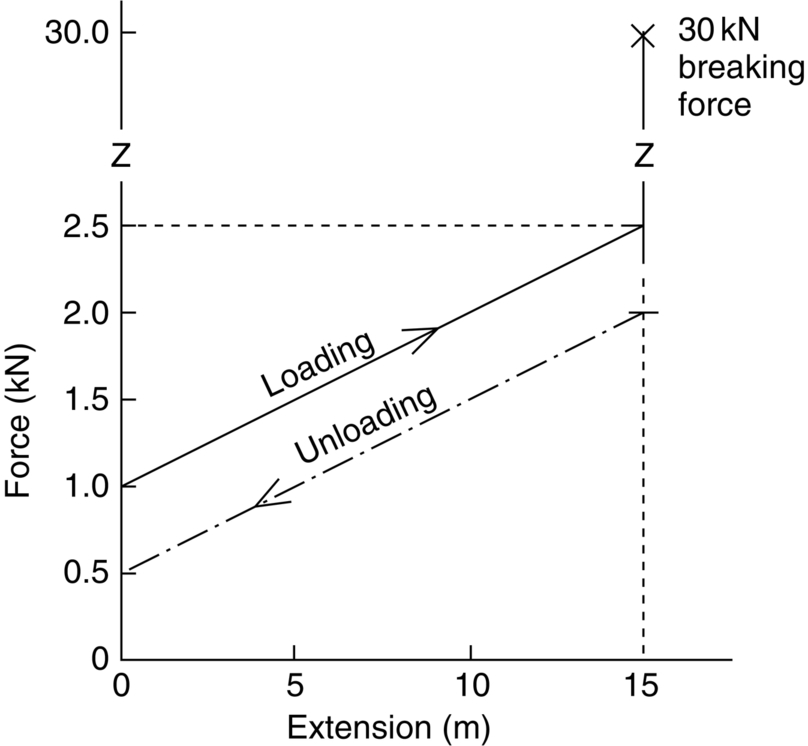
Worked Example
Examples
Answers
 . Values of σ are obtained by dividing the hardness values by 3. ɛn is the nominal strain given in the table plus 0.08.
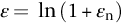
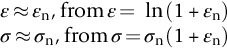
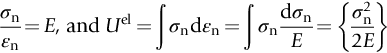
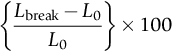
Revision of Terms and Useful Relations