This chapter has a two-fold objective. First, it introduces the nomenclature that will be used throughout the book. Second, it presents the basic mathematical theory necessary to describe nonlinear systems, which will help the reader to understand their rich set of behaviors. This will clarify several important distinctions between linear and nonlinear circuits and their mathematical representations.
We shall start with a brief review of linearity and linear systems, their main properties and underlying assumptions. A reader familiarized with the linear system realm can understand the limitations of the theoretical abstraction framed in the linearity mathematical concept, realizing its validity borders and so be prepared to cross them, i.e., to enter the natural world of nonlinearity. We will then introduce nonlinear systems and the responses that we should expect from them. After this, we will study one static, or memoryless, nonlinearity and a dynamic one, i.e., one that exhibits memory. This will then establish the foundations of nonlinear static and dynamic models and their basic extraction procedures.
The chapter is presented as follows: Section 1.1 is devoted to nomenclature and Section 1.2 reviews linear system theory. Sections 1.3 and 1.4 illustrate the types of behaviors found in general nonlinear systems and, in particular, in nonlinear RF and microwave circuits. Then, Sections 1.5 and 1.6 present the theory of nonlinear static and dynamic systems that will be useful to understand the nonlinear circuit simulation algorithms treated in Chapter 2 and the device modeling techniques of Chapters 3–6. Mathematics of nonlinear systems, and in particular dynamic ones, is not easy or trivial. So, we urge you to not feel discouraged if you do not understand it after your first read. What you will find in the next chapters will certainly help provide a physical meaning and practical usefulness to most of these sometimes abstract mathematical formulations. Finally, Section 1.7 closes this chapter with a brief conclusion.
1.1 Basic Definitions
We will frequently use the notion of model and system, so it is convenient to first identify these concepts.
1.1.1 Model
A model is a mathematical description, or representation, of a set of particular features of a physical entity that combines the observable (i.e., measurable) magnitudes and our previous knowledge about that entity. Models enable the simulation of a physical entity and so allow a better understanding of its observed behavior and provide predictions of behaviors not yet observed. As models are simplifications of the physically observable, they are, by definition, an approximation and restricted to represent a subset of all possible behaviors of the physical device.
1.1.2 System
As depicted in Figure 1.1, a system is a model of a machine or mechanism that transforms an input (excitation, or stimulus, usually assumed as a function of time), x(t), into an output (or response, also varying in time), y(t). Mathematically, it is defined as the following operator: y(t) = S[x(t)], in which x(t) and y(t) are, themselves, mathematical representations of the input and output measurable signals, respectively. Please note that, contrary to ordinary mathematical functions, which operate on numbers (i.e., that for a given input number, x, they respond with an output number, y = f(x)), mathematical operators map functions, such as x(t), onto other functions, y(t). So, they are also known as mathematical function maps. And, similar to what is required for functions, a particular input must be mapped onto a particular, unique, output.
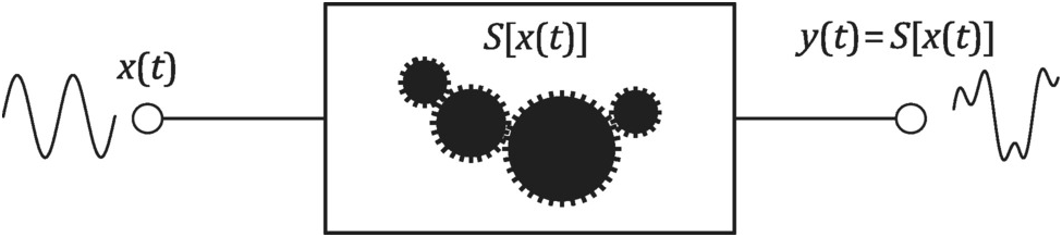
Figure 1.1 Illustration of the system concept.
When the operator is such that its response at a particular instant of time, y(t0), is only dependent on that particular input instant, x(t0), i.e., the system transforms each input value onto the corresponding output value, the operator is reduced to a function and the system is said to be static or memoryless. When, on the other hand, the system output cannot be uniquely determined from the instantaneous input only but depends on x(t0) and its x(t) past and future values, x(t ± τ), i.e., the system is now an operator of the whole x(t) onto y(t), we say that the system is dynamic or that it exhibits memory. (In practice, real systems cannot depend on future values because they must be causal.) For example, resistive networks are static systems, whereas networks that include energy storage elements (memory), such as capacitors, inductors or transmission lines, are dynamic.
Defined this way, this notion of a system can be used as a representation, or model, of any physical device, which can either be an individual component, a circuit or a set of circuit blocks. An interesting feature of this definition is that a system is nestable, i.e., it is such that a block (circuit) made of interconnected individual systems (circuit elements or components) can still be treated as a system. So, we will use this concept of system whenever we want to refer to the properties that we normally observe in components or circuits.
1.1.3 Time Invariance
Although the system response, y(t), varies in time, that does not necessarily mean that the system varies in time. The change in time of the response can be only a direct consequence of the input variation with time. This time-invariance of the operator is expressed by stating that the system reacts exactly in the same way regardless at which time it is subjected to the same input. That is, if the response to x(t) is y(t) = S[x(t)], and another test is made after a certain amount of time, τ, then the response will be exactly the same as before, except that now it will be naturally delayed by that same amount of time y(t − τ) = S[x(t − τ)]. This defines a time-invariant system. If, on the other hand, y(t − τ) ≠ S[x(t − τ)], then the system is said to be time-variant.
The vast majority of physical systems, and thus of electronic circuits, are time-invariant. Therefore, we will assume that all systems referred to in this and succeeding chapters are time-invariant unless otherwise explicitly stated.
After finalizing the study of this chapter, the reader may try Exercise 1.5 which constitutes a good example of how we can make use of this time-variance property for enabling us to treat, as a much simpler linear time-variant system, a modulator that is inherently nonlinear and time-invariant.
1.2 Linearity and the Separation of Effects
Now we will define a linear system as one that obeys superposition and recall how we use this property to determine the response of a linear system to a general excitation.
1.2.1 Superposition
A system is said to be linear if it obeys the principle of superposition, i.e., if it shares the properties of additivity and homogeneity.
The additivity property means that if y1(t) is the system response to x1(t), y1(t) = S[x1(t)], y2(t) is the system’s response to x2(t), y2(t) = S[x2(t)], and yT(t) is the response to x1(t) + x2(t), then
The additivity property is the mathematical statement that affirms that a linear system reacts to an additive composition of stimuli as an additive composition of responses, as if the system could distinguish each of the stimuli and treat them separately. In practical terms, this would mean that, if, in the lab, the result of an experiment with a cause x1(t) would produce an effect y1(t), and another, independent, experiment, on another cause x2(t), would produce y2(t), then, a third experiment, now made on a third stimulus x1(t) + x2(t), would produce a response that is the numerical summation of the two previously obtained effects y1(t) + y2(t).
On the other hand, the homogeneity property means that if α is a constant, then the response to αx(t) will be αy(t), i.e.,
The homogeneity property is the mathematical description of proportionality that says that an α times larger cause produces an α times larger effect. However, it does not necessarily state that the effects are proportional to their corresponding causes. For example, although the current and the voltage in a constant (linear) capacitance obey the homogeneity principle, they are not proportional to each other. In fact, since the current in a capacitor is given by (1.3), the current to a twice as large vc(t) will be twice as large as ic(t). However, that does not mean that ic(t) is proportional to vc(t), as can be readily noticed when vc(t) is a ramp in time and ic(t) is a constant.
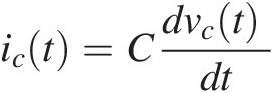 (1.3)
(1.3)In summary, linear systems obey the principle of superposition,
 (1.4)
(1.4)1.2.2 Response of a Linear System to a General Excitation
Superposition has very useful consequences that we now briefly review. They all revolve around that idea of the separation of effects, whereby we can expand any previously untested stimulus into a summation of previously tested excitations, making general predictions about the system responses.
1.2.2.1 Linear Response in the Time Domain
In the time domain, this means that, if we represent any input, x(t), as composed of the succession of its time samples, taken at regular intervals, Ts, of a constant sampling frequency fs = 1/Ts, so that they asymptotically produce the same effect of x(t), x(nTs)Ts,
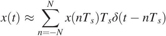 (1.5)
(1.5)in which δ(t − nTs)δt−nTs is the Dirac delta, or impulse, function centered at nTs, where n is the number of samples, (see Figure 1.2(a)), and we know the response of the system to one of these impulse functions of unity amplitude, h(t) = S[δ(t)]ht=Sδt (see Figure 1.2(b)), then we can readily predict the response to any arbitrary input x(t) as
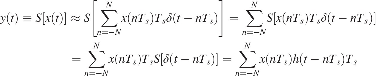 (1.6)
(1.6)by simply making use of the additivity and homogeneity properties (as shown in Figure 1.2(c)). Expression (1.6) is exact in the limit when the sampling interval, Ts, tends to zero and N tends to infinity, becoming the well-known convolution integral:
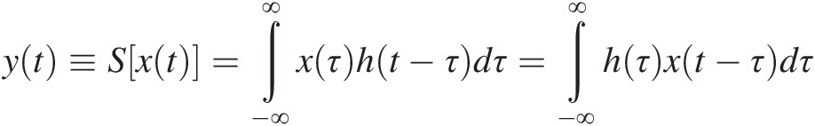 (1.7)
(1.7)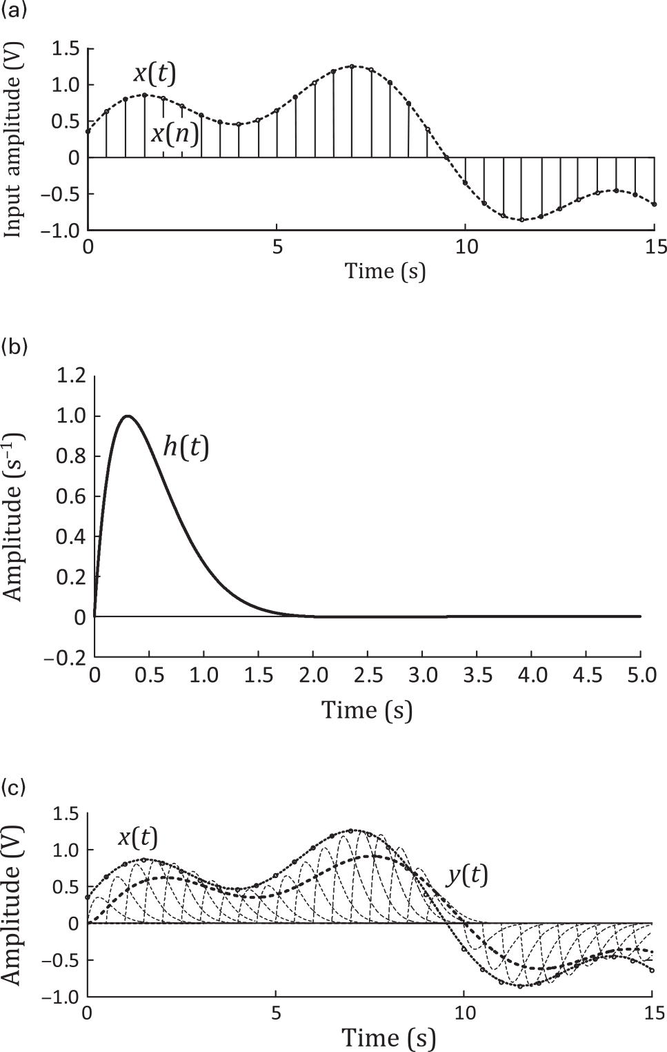
Figure 1.2. Response, y(t)yt, of a linear dynamic and time-invariant system to an arbitrary input, x(t)xt, when this stimulus is expanded in a summation of Dirac delta functions. (a) Input expansion with the base of delayed Dirac delta functions x(n) = x(nTs)δ(t − nTs)xn=xnTsδt−nTs. (b) Impulse response of the system, h(t) = S[δ(t)]ht=Sδt. (c) Response of the system to x(t)xt, y(t) = S[x(t)]yt=Sxt.
1.2.2.2 Linear Response in the Frequency Domain
So, in time domain, we only needed to know the system response to one input basis function – the impulse response, h(t) = S[δ(t)]ht=Sδt, to be able to predict the response to any other arbitrary input. Similarly, in the frequency domain we only need to know the response to one input basis function, the cosine, although tested at all frequencies, to predict the response to any arbitrary periodic input.
Actually, since the cosine can be given as the additive combination of two complex exponentials
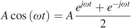 (1.8)
(1.8)from a mathematical viewpoint, we only need to know the response to that basic complex exponential. This response can be obtained from (1.7) as
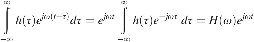 (1.9)
(1.9)in which H(ω)Hω is the Fourier transform of h(τ)hτ. This is an interesting result that tells us that the response to an arbitrary x(t) can be easily computed by summing up the Fourier components of that input scaled by the system’s response to each particular frequency. Indeed, if R(ω)Rω is the frequency-domain Fourier representation of a time-domain signal r(t), so that
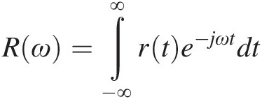 (1.10a)
and
 (1.10b)
then, the substitution of (1.10) into (1.7) would lead to
where Y(ω)Yω can be related to y(t) – as X(ω)Xω is related to x(t) – by the Fourier transform of (1.10). This expression tells us the following two important things.
First, the time-domain convolution of (1.7) between the input, x(t), and the impulse response, h(τ)hτ, becomes the product of the frequency-domain representation of these two entities, X(ω)Xω and H(ω)Hω, respectively.
Second, the response of a linear time-invariant system to a continuous-wave (CW) signal (an unmodulated carrier of frequency ωω, specifically cos (ωt)cosωt) is another CW signal of the same frequency with, possibly, different amplitude and phase. Consequently, the response to a signal of complex spectrum will only have frequency-domain components at the frequencies already present at the input. A time-invariant linear system is incapable of generating new frequency components or of performing any qualitative transformation of the input spectrum.
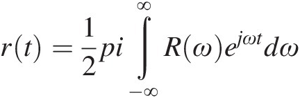
Finally, equation (1.11) tells us that, in the same way we only needed to know the system’s impulse response to be able to predict the response to any arbitrary stimulus in the time domain, we just need to know H(ω) to predict the response to any arbitrary periodic input described in the frequency domain. As an illustration, Figure 1.3 depicts the measured transfer function S21(ω), in amplitude and phase, of a microwave filter.
1.3 Nonlinearity: The Lack of Superposition
As all of us have been extensively taught and trained in working with linear systems, and with the additivity and homogeneity properties being so intuitive, we may easily fall into the trap of believing that these should be properties naturally inherent to all physical systems. But this is not the case. In fact, most of macroscopic physical systems behave very differently from linear systems, i.e., they are not linear. Actually, we use the term nonlinear systems to identify them.
Since we have been making the effort to define all important concepts used so far, we should start by defining a nonlinear system. But that is not a straightforward task as there is no general definition for these systems. There is only the unsatisfying definition of defining something by what it is not: a nonlinear system is one that is not linear, i.e., a nonlinear system is one that does not obey the principle of superposition. This is an intriguing, but also revealing, situation, which tells us that if linear systems are the ones that obey a precise mathematical principle, nonlinear systems are all the other ones. Hence, from an engineering standpoint the relevant question to be answered is: Are nonlinear systems often seen, or used, in practice? To demonstrate their importance, let us try a couple of very common, RF electronic examples. But, before these, the reader may want to try the two simpler examples discussed in Exercises 1.1–1.4.
In this example we will show that any active device must be nonlinear.
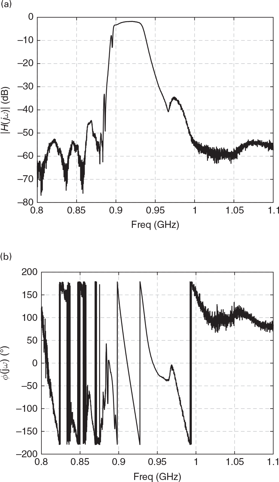
As a first step, we will show that all active devices depend on two different excitations. One is the input signal and the other is the dc power supply. This means, as illustrated in Figure 1.4, that amplifiers are transducers that convert the power supplied by a dc power source into output signal power, i.e. they convert dc into RF power.
Now, as the second step in our attempt to prove that any active device must be nonlinear, let us assume, instead, that it could be linear. Then, it would have to obey the additivity property, which means that the response to each of the inputs, the signal and the power supply, should be determined separately. That is, the response to the auxiliary supply and to the signal should be obtained as if the other stimulus would not exist. And we would come back to an amplifier that could amplify the signal power without requiring any auxiliary power, thus violating the energy conservation principle.
Although this argument seems quite convincing, it raises a puzzling question, because, if it is impossible to produce amplifiers without requiring nonlinearity, we should be magicians as we all have already seen and designed linear amplifiers. So, how can we overcome this paradox?
Figure 1.4 Illustration of the power flow in a transducer or amplifier.
According to the power flow shown in Figure 1.4, where PinPin, PoutPout, PdcPdc and PdissPdiss are, respectively, the signal input and output powers, the supplied dc power and the dissipated power (herein assumed as all forms of energy that are not correlated with the information signal, such as heat, harmonic generation, intermodulation distortion, etc.), the amplifier gain, GG, can be defined by
 (1.12)
And this G must be constant and independent of PinPin for preserving linearity.
Imposing the energy conservation principle to this transducer results in
from which the following constraint can be found for the gain:
 (1.14)
Since PdissPdiss cannot decrease below zero (100% dc-to-RF conversion efficiency) and PdcPdc must be limited (as is proper from real power sources), G(Pin)GPin cannot be kept constant but must decrease beyond a certain maximum Pin.
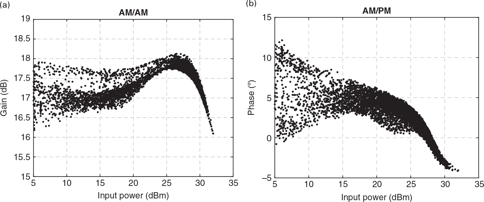
In RF amplifiers, this gain decrease with input signal power is called gain compression. In practice, amplifiers not only exhibit a gain variation when their input amplitude changes, but also an input-dependent phase shift. This is particularly important in RF amplifiers intended to process amplitude modulated signals as this input modulation is capable of inducing nonlinear output amplitude and phase modulations. These are the well-known AM/AM and AM/PM nonlinear distortions, often plotted as shown in Figure 1.5(a) and (b), respectively.
This analysis shows that linearity can only be obeyed at sufficiently small signal levels, and that it is only a matter of excitation amplitude to make an apparently linear amplifier expose its hidden nonlinearity.
Actually, this study provided us a much deeper insight of linearity and linear systems. Linearity is what we obtain when looking only at the system’s input to output signal mapping (leaving aside the dc-to-RF energy conversion process) and when the signal is a very small perturbation of the dc quiescent point. So, linear systems are the conceptual mathematical model for the behaviors obtained from analytic operators (i.e., that are continuous and infinitely differentiable mappings), when these are excited with signals whose amplitudes are infinitesimally small as compared with the magnitude of the quiescent points. And it is under this small-signal operation regime that the linear approximation is valid. We will come back to this important concept later.
Example 1.2 A Sinusoidal Oscillator
A sinusoidal oscillator is another system that depends on nonlinearity to operate. Although in basic linear system analysis we learned how to predict the stable and unstable regimes of amplifiers, and so to predict oscillations, we were not told the complete story. To understand why, we can just use the above results on the analysis of the amplifier and recognize that, by definition, an oscillator is a system that provides an output even without an input. That is, contrary to an amplifier that is a nonautonomous, or forced, system, an oscillator is an autonomous one. So, if it would not rely on any external source of power, it would violate the energy conservation principle. Like an amplifier, it is, instead, a transducer that converts energy from a dc power supply into signal power at some frequency ω. Hence, like the amplifier, it must rely on some form of nonlinearity. But, unlike the amplifier, in which we have shown that, seen from the input signal to the output signal, it could behave in an approximately linear way, we will now show that not even this is possible in an oscillator.
To see why, consider the following linear differential equation of constant (i.e., time-invariant) coefficients – one of the most common models of linear systems:
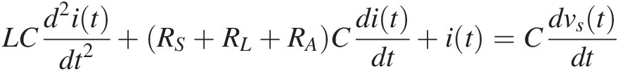 (1.15)
which describes the loop current, i(t), sinusoidal oscillations of a series RLC circuit when the excitation vanishes, vs(t) = 0vst=0. The proof that this equation is indeed the model of a linear time-invariant system is left as an exercise for the reader (see Exercise 1.6).
This RLC circuit is assumed to be driven by an active device whose model for the power delivered to the network is the negative resistance RA, and to be loaded by the load resistance RL and the inherent LC tank losses RS. It can be shown that the solution of this equation, when vs(t) = 0vst=0, is of the form
where λ=RS+RL+RA2L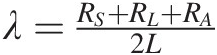 and ω=1LC−λ2
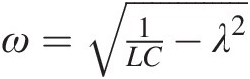 .
.
The first curious result of this linear oscillator model is that it does not provide any prediction for the oscillation amplitude A as if A could be any arbitrary value. The second is that, to keep a steady-state oscillation, i.e., one whose amplitude does not decay or increase exponentially with time, λλ must be exactly (i.e., with infinite precision) zero, or RA = − (RS + RL)RA=−RS+RL something our engineering common sense finds hard to believe. Both of these unreasonable conditions are a consequence of the absence of any energy constraint in (1.15), which, itself, is a consequence of the performed linearization. In practice, what happens is that the active device is nonlinear, its negative resistance is not constant but an increasing function of amplitude, RA(A) = − f(A)RAA=−fA, so that a negative feedback process keeps the oscillation amplitude constant at A = f−1(RS + RL)A=f−1RS+RL, in which f−1(.)f−1. represents the inverse function of f(.)f..
Although nonlinearity is often seen as a source of perturbation, referred to with many terms, such as harmonic distortion, nonlinear cross-talk, desensitization, or intermodulation distortion, it plays a key role in wireless communications. As a matter of fact, these two examples, along with the amplitude modulator of Exercises 1.3–1.5, show that nonlinearity is essential for amplifiers, oscillators, modulators, and demodulators. And since wireless telecommunication systems depend on these devices to generate RF carriers, translate information base-band signals back and forth to radio-frequency frequencies (reducing the size of the antennas), and provide amplification to compensate for the free-space path loss, we easily conclude that without nonlinearity wireless communications would be impossible. As an illustration, Figure 1.6 shows the block diagram of a wireless transmitter where the blocks from which nonlinearity should be expected are put in evidence.
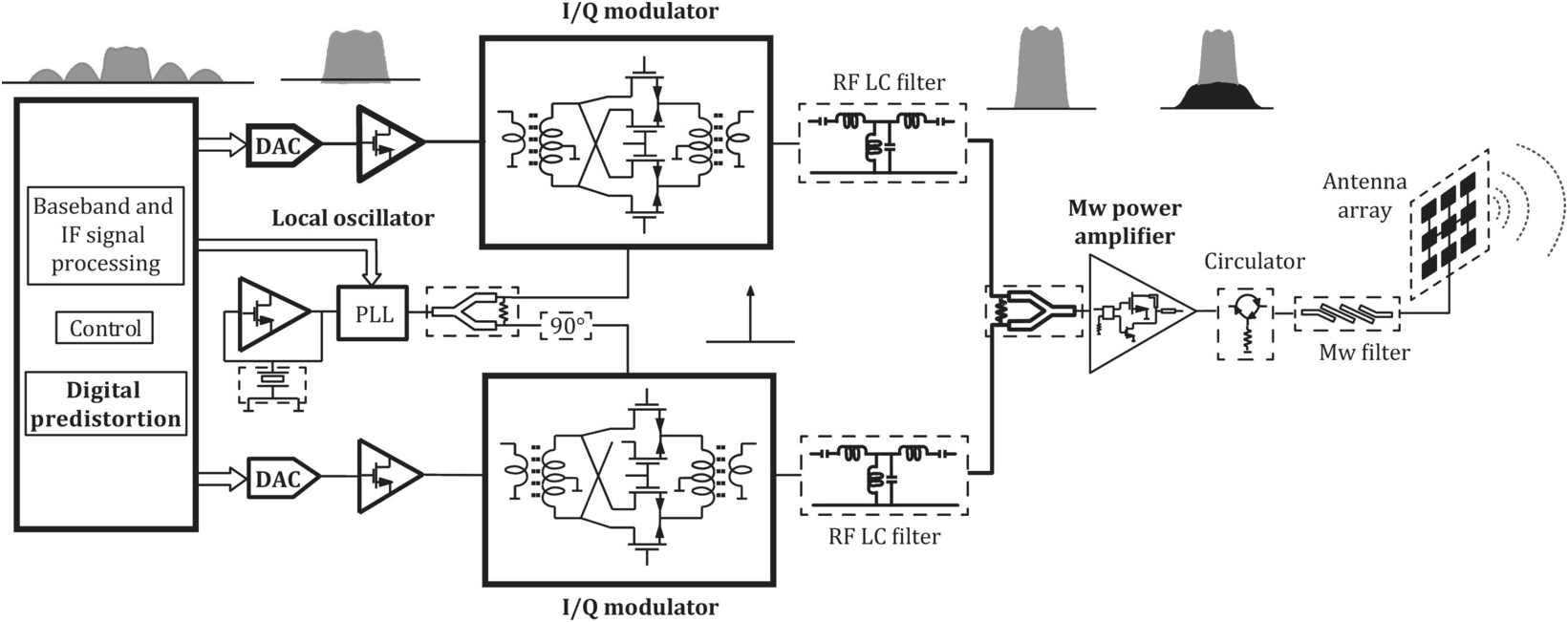
Figure 1.6 Block diagram of a wireless transmitter where the blocks from which nonlinearity is expected are highlighted: linear blocks are represented within dashed line boxes whereas nonlinear ones are drawn within solid line boxes.
1.4 Properties of Nonlinear Systems
This section illustrates the multiplicity of behaviors that can be found in nonlinear dynamic systems. Although a full mathematical analysis of those responses does not constitute a key objective of this chapter, we will nevertheless base our tests in a simple circuit so that each of the observed behaviors can be approximately explained by relating it to the circuit topology and components.
The analyses will be divided in forced and autonomous regimes, like the ones found in amplifiers or frequency multipliers and oscillators, respectively. However, to obtain a more applied view of these responses we will further group forced regimes in responses to CW and modulated excitations.
1.4.1 An Example of a Nonlinear Dynamic Circuit
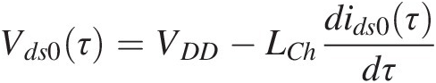
To start exploring some of the basic properties of nonlinear systems, we will use the simple (conceptual) amplifier shown in Figure 1.7.
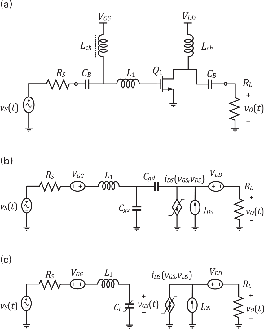
Figure 1.7 (a) Conceptual amplifier circuit used to illustrate some properties of forced nonlinear systems. (b) Equivalent circuit when the dc block capacitors and the dc feed inductances are substituted by their corresponding dc sources. (c) Simplified unilateral circuit after Cgd was reflected to the input via its Miller equivalent.
In order to preserve the desired simplicity, enabling us to qualitatively relate the obtained responses to the circuit’s model, we will assume that the input and output block capacitors, CB, and the RF bias chokes, LCh, are short-circuits and open circuits to the RF signals, respectively. Therefore, the dc blocking capacitors can be simply replaced by two ideal dc voltage sources, the gate RF choke can be neglected, and the drain choke must be replaced by a dc current source that equals the average iDS(t) current, IDS. This is illustrated in Figure 1.7(b). Furthermore, we will also assume that the FET’s feedback capacitor, Cgd, can be replaced by its input and output reflected Miller capacitances, which value Cgd_in = Cgd(1−Av) and Cgd_out = Cgd(Av−1)/Av, respectively. Assuming that the voltage gain, Av, is negative and much higher than one (rigorously speaking, much smaller than minus one) the total FET’s input capacitance, Ci, will be approximately given by Ci = Cgs + Cgd|Av| while the output capacitance, Co, will equal Cgd, being thus negligible. Under these conditions, the schematic of Figure 1.7(b) becomes the one shown in Figure 1.7(c), whose analysis, using Kirchhoff’s laws, leads to
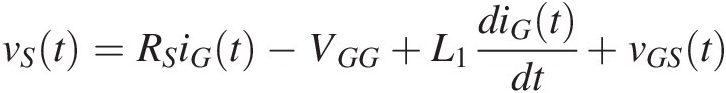 (1.17)
and
in which iGt=CidvGStdt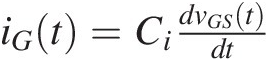 is the gate current flowing through Ci and iDS(t)iDSt is the FET’s drain-to-source current. This drain current is assumed to be some suitable static nonlinear function of the gate-to-source voltage, vGS(t), and drain-to-source voltage, vDS(t).
In case vDS(t) is kept sufficiently high so that vDS(t) >> VK, the FET’s knee voltage, iDS(t) can be considered only dependent on the input voltage, iDS(vGS). Using these results in (1.17), the differentiation chain rule leads to a second order differential equation
 (1.19)
whose solution, vGS(t)vGSt, allows the determination of the amplifier output voltage as
1.4.2 Response to CW Excitations
Because of its central role played in RF circuits, we will first start by identifying the responses to sinusoidal, or CW, (plus the dc bias) excitations. Hence, our amplifier is described by a circuit that includes two nonlinearities: iDS(vGS,vDS) that is static and Ci, a nonlinear capacitor, which, depending on the voltage gain, evidences its nonlinearity when the amplifier suffers from iDS(vGS,vDS) induced gain compression.
Figure 1.8 shows the drain-source voltage evolution in time, vDS(t), for three different CW excitation amplitudes, while Figure 1.9 depicts the respective spectra. Under small-signal regime, i.e, small excitation amplitudes, in which the FET is kept in the saturation region and vgsvgs (the signal component of the composite vGS voltage defined by vgs ≡ vGS − VGSvgs≡vGS−VGS and, in this case, VGS = VGGVGS=VGG) is so small that iDSvGSvDS≈IDS+gmvgs+gm2vgs2+gm3vgs3≈IDS+gmvgs , the amplifier presents an almost linear response without any other harmonics than the dc and the fundamental component already present at the input. As we increase the excitation amplitude, the vGS(t) and vDS(t) voltage swings become sufficiently large to excite the FET’s iDS(vGS,vDS) cutoff (vGS(t) < VT, the FET’s threshold voltage) and knee voltage nonlinearities (vDS(t) ≈ VK), and the amplifier starts to evidence its nonlinear behavior, producing other frequency-domain harmonic components or time-domain distorted waveforms.
Figure 1.8 vDS(t) voltage evolution in time for three different CW excitation amplitudes. Note the distorted waveforms arising when the excitation input is increased.
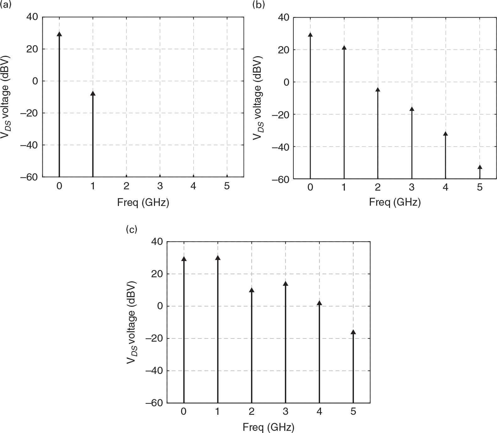
Figure 1.9 Vds(ω) spectrum for three different CW excitation amplitudes. Note the increase in the harmonic content with the excitation amplitude.
In a cubic nonlinearity as the one above used for the dependence of iDS on vGS, this means that a sinusoidal excitation, vs(t) = Acos(ωt)vst=Acosωt, produces a gate-source voltage of vgs(t) = |Vgs(ω)| cos (ωt + ϕi)vgst=Vgsωcosωt+ϕi, in which
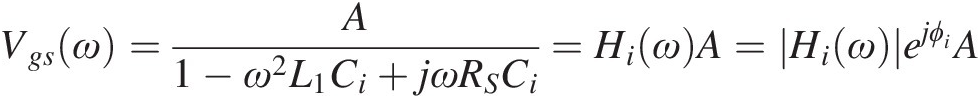 (1.21)
produces the following ids(t) response:
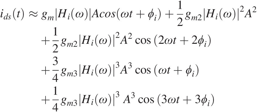 (1.22)
which evidences the generation of a linear component, proportional to the input stimulus, a quadratic dc component and second and third harmonics, beyond a cubic term at the fundamental. Actually, it is this fundamental cubic term that is responsible for modeling the amplifier’s gain compression since the equivalent amplifier transconductance gain is
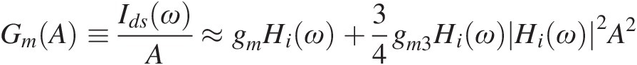 (1.23)
i.e., is dependent on the input amplitude.
In communication systems, in which an RF sinusoidal carrier is modulated with some amplitude and phase information (the so-called complex envelope [1]), such a gain variation with input amplitude has always deserved particular attention, since it describes how the input amplitude and phase information are changed by the amplifier. This defines the so-called AM/AM and AM/PM distortions. That is what is represented in Figures 1.10 and 1.11, in which the input–output fundamental carrier amplitude and phase (with respect to the input phase reference) is shown versus the input amplitude. When the output voltage waveform becomes progressively limited by the FET’s nonlinearities, its corresponding gain at the fundamental component gets compressed and its phase-lag reduced. Indeed, when the voltage gain is reduced, so is the Cgd Miller reflected input capacitance, and thus Ci. Hence, the phase of Hi(ω) increases, and consequently, the vGS(t) fundamental component shows an apparent phase-lead (actually a reduced phase-lag), revealed as the AM/PM of Figure 1.11.
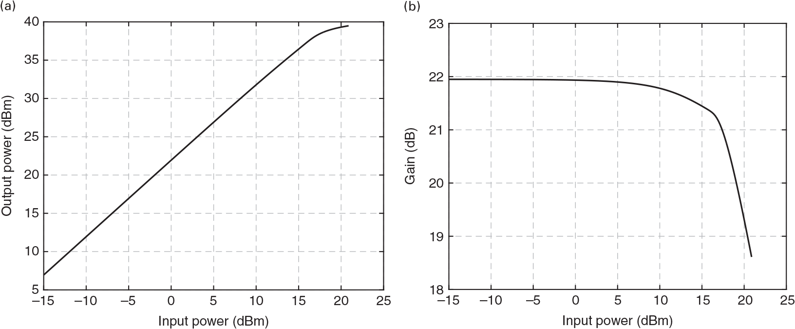
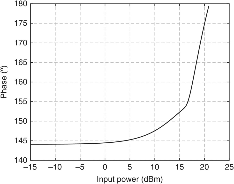
Figure 1.11 Response to CW excitations: AM/PM characteristic.
What happens in real amplifiers (see, for example, [2]) is that, because of the circuit nonlinear reactive components, or, as was here the case, because of the interactions between linear reactive components (Cgd) and static nonlinearities (iDS(vGS,vDS), which manifests itself as a nonlinear voltage gain, Av), the equivalent gain suffers a change in both magnitude and phase manifested under CW excitation as AM/AM and AM/PM.
1.4.3 Response to Multitone or Modulated Signals
The extension of the CW regime to a modulated one is trivial, as long as we can assume that the circuit responds to a modulated signal like
without presenting any memory to the envelope. This means that the circuit treats our modulated carrier as a succession of independent CW signals of amplitude a(τ) and phase ϕ(τ). That is, we are implicitly assuming that the envelope varies in a much slower and uncorrelated way – as compared to the carrier – (the narrow bandwidth approximation), as if the RF carrier would evolve in a fast time t while the base-band envelope would evolve in a much slower time τ. In that case, for example, a two-tone signal of frequencies ω1 = ωc−ωm and ω2 = ωc + ωm, i.e., whose frequency separation is 2ωm and is centered at ωc, and in which ωc >> ωm, can be seen as a double sideband amplitude modulated signal of the form
Applied to our nonlinear circuit, this modulated signal will generate several out-of-band and in-band distortion components centered at the carrier harmonics and the fundamental carrier, respectively.
This is illustrated in Figure 1.12, where both the time-domain envelope waveform and frequency-domain spectral components of our amplifier response to a two-tone signal of fc = 1 GHz and fm = 10 kHz, are represented.
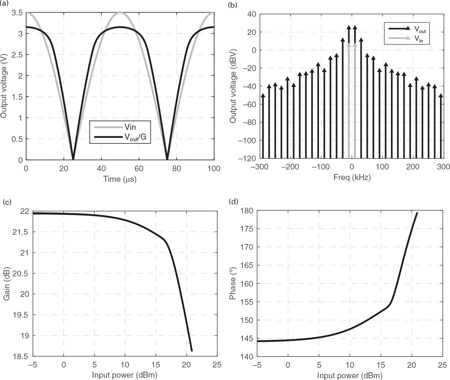
Figure 1.12 (a) Time-domain envelope waveform and (b) frequency-domain envelope spectra of our nonlinear circuit’s response to a two-tone signal; (c) and (d) represent, respectively, the amplitude and phase profiles of the amplifier gain defined as the ratio of the instantaneous output to the instantaneous input complex envelopes.
In fact, still using the cubic nonlinearity of iDS(vGS)iDSvGS and the input transfer function of (1.21), we would obtain an output response of the form
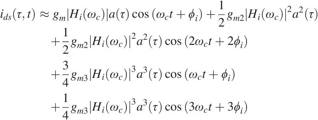 (1.26)
which is composed of the following terms:
(i) gm ∣ Hi(ωc) ∣ a(τ) cos (ωct + ϕi) = gm ∣ Hi(ωc) ∣ Acos(ωmτ) cos (ωct + ϕi)gm∣Hiωc∣aτcosωct+ϕi=gm∣Hiωc∣Acosωmτcosωct+ϕi is the two-tone fundamental linear response located at ω1 = ωc−ωm and ω2 = ωc + ωm;
(ii) 12gm2Hiωc2a2τ
 is located near the 0-order harmonic frequency of the carrier, and is composed of a tone at dc, of amplitude 14gm2Hiωc2A2
 – representing the input-induced bias change from the quiescent point to the actual dc bias operating point – and another tone at ω2−ω1 or 2ωm, of amplitude 14gm2Hiωc2A2
 , representing the dc bias fluctuation imposed by the time-varying carrier amplitude.
(iii) 12gm2Hiωc2a2τcos2ωct+2ϕi
 is the second harmonic distortion of the amplifier and is composed of three tones at 2ω1 = 2ωc−2ωm and 2ω2 = 2ωc + 2ωm, of amplitude 18gm2Hiωc2A2
 , and a center tone at ω1 + ω2 = 2ωc, of amplitude 14gm2Hiωc2A2
 ;
;
(iv) 34gm3HiωcHiωc2a3τcosωct
 are again fundamental components located at ω1 = ωc−ωm and ω2 = ωc + ωm, of amplitude 932gm3Hiωc3A3
 , plus two in-band distortion sidebands located at 2ω1−ω2 = ωc−3ωm and 2ω2−ω1 = ωc + 3ωm, of amplitude 332gm3Hiωc3A3
 ;
;
and
(v) 14gm3Hi3ωca3τcos3ωct
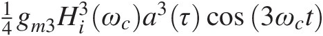 the third harmonic distortion of the amplifier, composed of four tones at 2ω1 + ω2 = 3ωc−ωm and 2ω2 + ω1 = 3ωc + ωm, of amplitude 332gm3Hiωc3A3
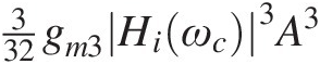 , and two sidebands at 3ω1 = 3ωc−3ωm and 3ω2 = 3ωc + 3ωm, of amplitude 132gm2Hiωc3A3
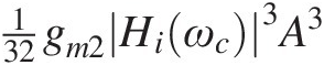 .
.
As the modulation complexity is increased from a sinusoid to a periodic signal, the amplifier response would still be composed by these frequency clusters located at each of the carrier harmonics. A more detailed treatment of this multitone regime can be found in the technical literature, e.g., [3–5]. Because the common frequency separation of the tones of these clusters is inversely proportional to the modulation period, 2π/ωm, a real modulated signal – which is necessarily aperiodic or with an infinite period – produces a spectrum that is composed of continuous bands centered at each of the carrier harmonics. Figure 1.13 illustrates a response to such a real wireless communications signal.
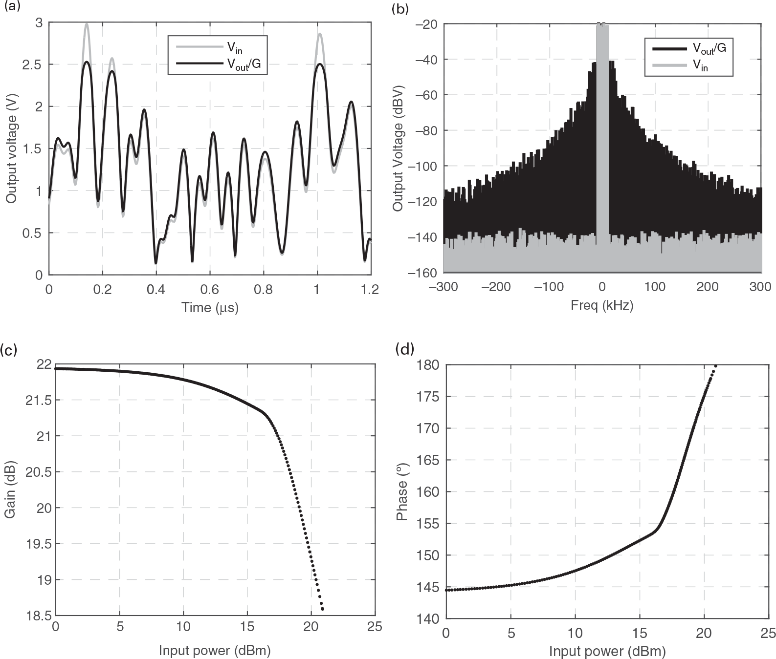
Figure 1.13 (a) Time-domain envelope waveform and (b) frequency-domain envelope spectrum of our nonlinear circuit’s response to a 20 kHz bandwidth OFDM wireless signal; (c) and (d) represent, respectively, the amplitude and phase profiles of the amplifier gain defined as the ratio of the instantaneous output to the instantaneous input complex envelopes.
If we now consider a progressively faster envelope, in which the amplifier has not enough time to reach the steady-state before its excitation amplitude or phase changes significantly, this narrowband approximation ceases to be valid and the amplifier exhibits memory to the envelope. This may happen either because the input transfer function Hi(ω) varies significantly within each of the harmonic clusters, or because the LCh and CB bias network elements can no longer be considered short and open circuits, respectively, for the base-band components (of type (ii) above) of this wideband envelope. This means that the response to a particular CW excitation is no longer defined by its instantaneous (to the envelope) amplitude or phase, but also depends on their past envelope states. For example, as the amplitude and phase changes can no longer be entirely defined by the input excitation amplitude, but are different if the envelope stimulus is rising or falling, the AM/AM and AM/PM exhibit hysteresis loops as the ones previously shown in the measured data of Figure 1.5 and now illustrated again in Figure 1.14. Envelope memory effects is a nontrivial topic, in particular concerning nonlinear power amplifier distortion and linearization studies as can be seen in the immense literature published on this subject [4], [6–9].
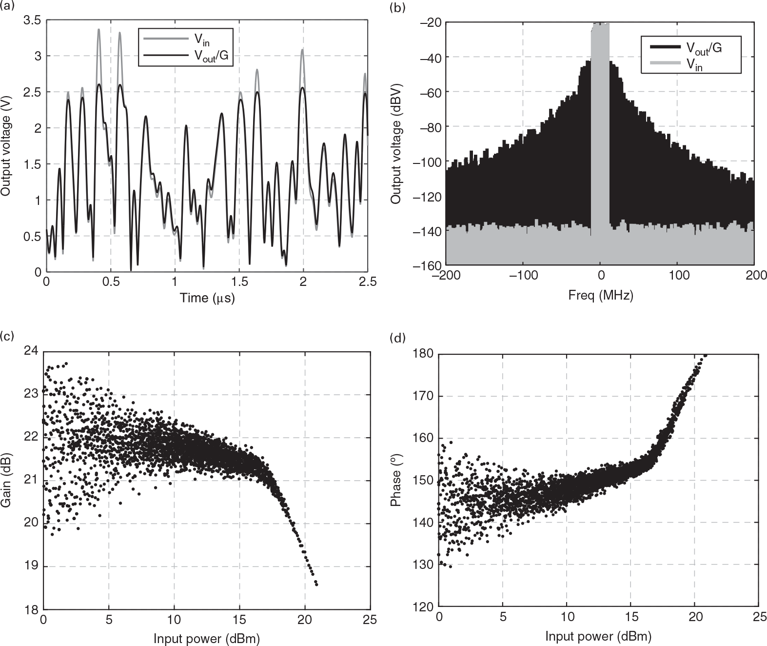
Figure 1.14 (a) Time-domain envelope waveform and (b) frequency-domain envelope spectra of our nonlinear circuit’s response to a OFDM wireless signal but now with a much wider bandwidth of 20 MHz; (c) and (d) represent, respectively, the amplitude and phase profiles of the amplifier gain defined as the ratio of the instantaneous output to the instantaneous input complex envelopes.
In our simple circuit, the main source of these envelope memory effects is the 12gm2Hiωc2a2τ ids0(τ) bias current fluctuation in the drain RF choke inductance, which generates a Vds0(τ) drain bias voltage variation, and thus gain change as is shown in Figure 1.14 [10]. However, as this Vds0(τ) variation is given by
 (1.27)
there is a gain reduction (increase) when the amplitude envelope is rising (falling) in time, with respect to what would be expected from a memoryless, or static, response.
1.4.4 Autonomous and Forced Responses from an Unstable Circuit
Now, we will address some of the properties of another important class of nonlinear regimes: the autonomous ones, i.e., regimes capable of generating new frequencies without any excitation. For that, we will use the forced Armstrong or Meissner oscillator [11] because it combines a surprising simplicity with an enormous diversity of effects. Actually, this simple oscillator circuit was invented in the first years of radio, when electronic circuits were implemented with triode tubes. When triodes were replaced by solid-state devices, such as the field-effect transistor, this oscillator acquired the topology shown in Figure 1.15.
This oscillator can be easily distinguished from the above studied amplifier since feedback is no longer any undesirable or parasitic effect but constitutes an essential ingredient of its operation. In this case, the feedback path is provided by the mutual inductor M that couples the input and output circuits of what can be seen as our previous ordinary amplifier.
There are two different types of autonomous regimes, periodic and aperiodic ones. Autonomous periodic regimes are what we normally expect from RF oscillators, while chaotic regimes are strange oscillatory phenomena that are aperiodic, but deterministic, i.e., they cannot be attributed to random noise fluctuations [12–14].
Then, a steady-state periodic oscillatory regime can still be perturbed by an external forcing signal to create a multitude of new phenomena, from phase-locked oscillations, analog frequency division, or self-oscillating mixing [15].
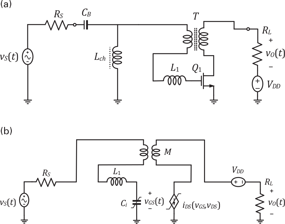
1.4.4.1 Autonomous Periodic Regime
Setting vS(t) = 0, i.e., eliminating any possible external excitation, we obtain the periodic (nearly sinusoidal) autonomous regime depicted in Figure 1.16. In Figure 1.16 (a), we can see the vgs(t) voltage evolution with time, which shows that, because the circuit is unstable in its quiescent point, it evolves from its dc quiescent point toward its sinusoidal steady-state regime.
Figure 1.16 (b) constitutes another commonly adopted alternative representation known as the phase-portrait. It is a graphic of the trajectory, or orbit, of the circuit or system state in the phase-space, i.e., in the state-variables that describe the system. In our second order system, these are the two state-variables of the differential equation that governs this response, vgs(t) and its first derivative in time, dvgs(t)/dt, of Eq. (1.18). In the phase-portrait, you can see that the system evolution in time is such that it starts with a null vgs(t), with null derivative (a dc point) and evolves to a cyclic trajectory, also known as a limit cycle, of 2 V amplitude and about 2.5 × 10⁹ Vs−1 dvgs(t)/dt amplitude. This phase-portrait also indicates that the steady state is periodic – as it tends to a constant trajectory, also known as an attractor – and nearly sinusoidal, but not purely sinusoidal. Indeed, if the steady state was a pure sinusoid, i.e., without any harmonics, the steady-state orbit would have to be a circle or an ellipse, depending on the x, vGS(t), and y, dvGS(t)/dt, relative scales.
Figure 1.17 presents the corresponding spectrum. Please note that, in the steady state, this periodic waveform is composed of discrete lines at multiples of the fundamental frequency, 200 MHz.
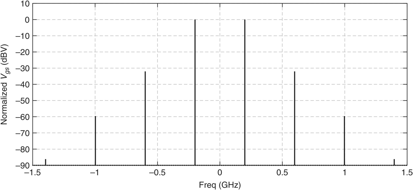
Figure 1.17 Spectrum of the vgs(t) voltage when the circuit operates in an oscillatory autonomous regime.
1.4.4.2 Forced Regime over an Oscillatory Response
To conclude this section on the type of responses we should expect from a nonlinear circuit, we now reduce the amount of feedback, i.e., M. As the feedback is now insufficient to develop an autonomous regime, the circuit is stable at its quiescent point. However, when forced with a sufficiently large excitation, it may develop parasitic oscillations as shown in Figures 1.18 and 1.19.
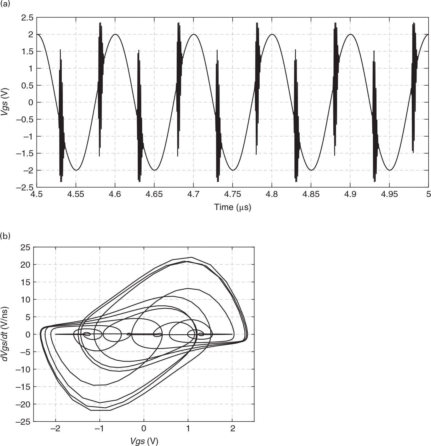
Figure 1.18 (a) vgs(t) voltage in the time domain and (b) its corresponding phase-portrait when the circuit is under a sinusoidal excitation but is evidencing parasitic oscillations.
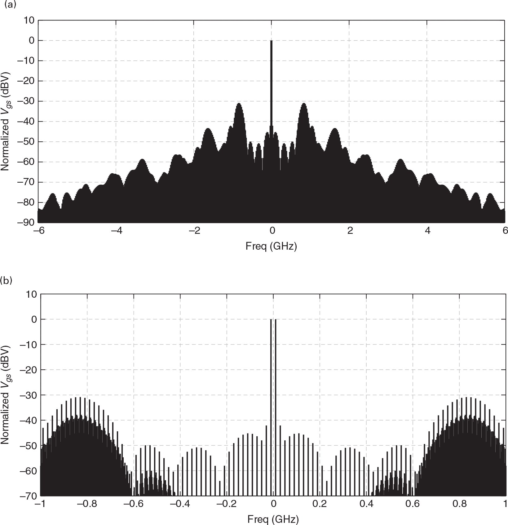
Figure 1.19 (a) Wide span and (b) narrow span spectrum of the vgs(t) voltage when the circuit is operating as an amplifier but exhibiting parasitic oscillations.
As the circuit is on the edge of instability, it can only develop and sustain the parasitic oscillation for a very particular excitation amplitude. However, there are also cases in which both the forced and autonomous regimes can be permanent and the amplifier/oscillator becomes an injection locked oscillator or a self-oscillating mixer depending on the relation of the frequencies of the excitation and of the oscillatory autonomous regime.
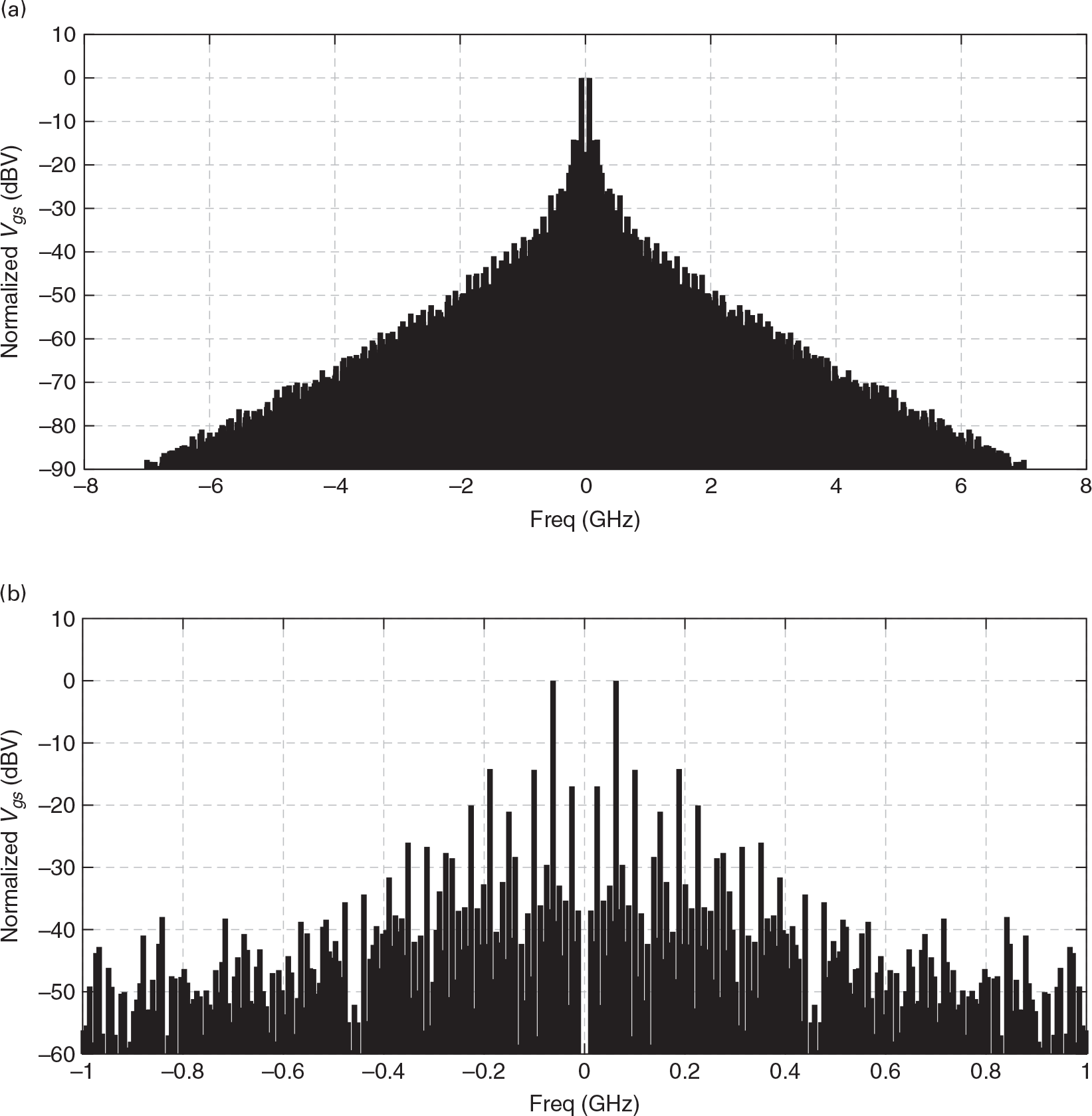
However, intended to illustrate the variety of different response types possible in nonlinear dynamic circuits, Figures 1.20 and 1.21 correspond to none of the referred cases. Now, the interaction between the amplitude and frequency of the excitation and of the oscillator itself makes it develop a regime that is neither periodic (indicative of injection locking) nor double periodic (indicative of mixing), but completely aperiodic: a chaotic regime. As shown in Figures 1.20 and 1.21, the regime is nearly periodic but not exactly periodic, as the attractor is not a closed curve that repeats itself indefinitely. Consequently, the spectrum is now filled in with an infinite number of spectral lines spaced infinitesimally closely, i.e., it is a continuous spectrum.
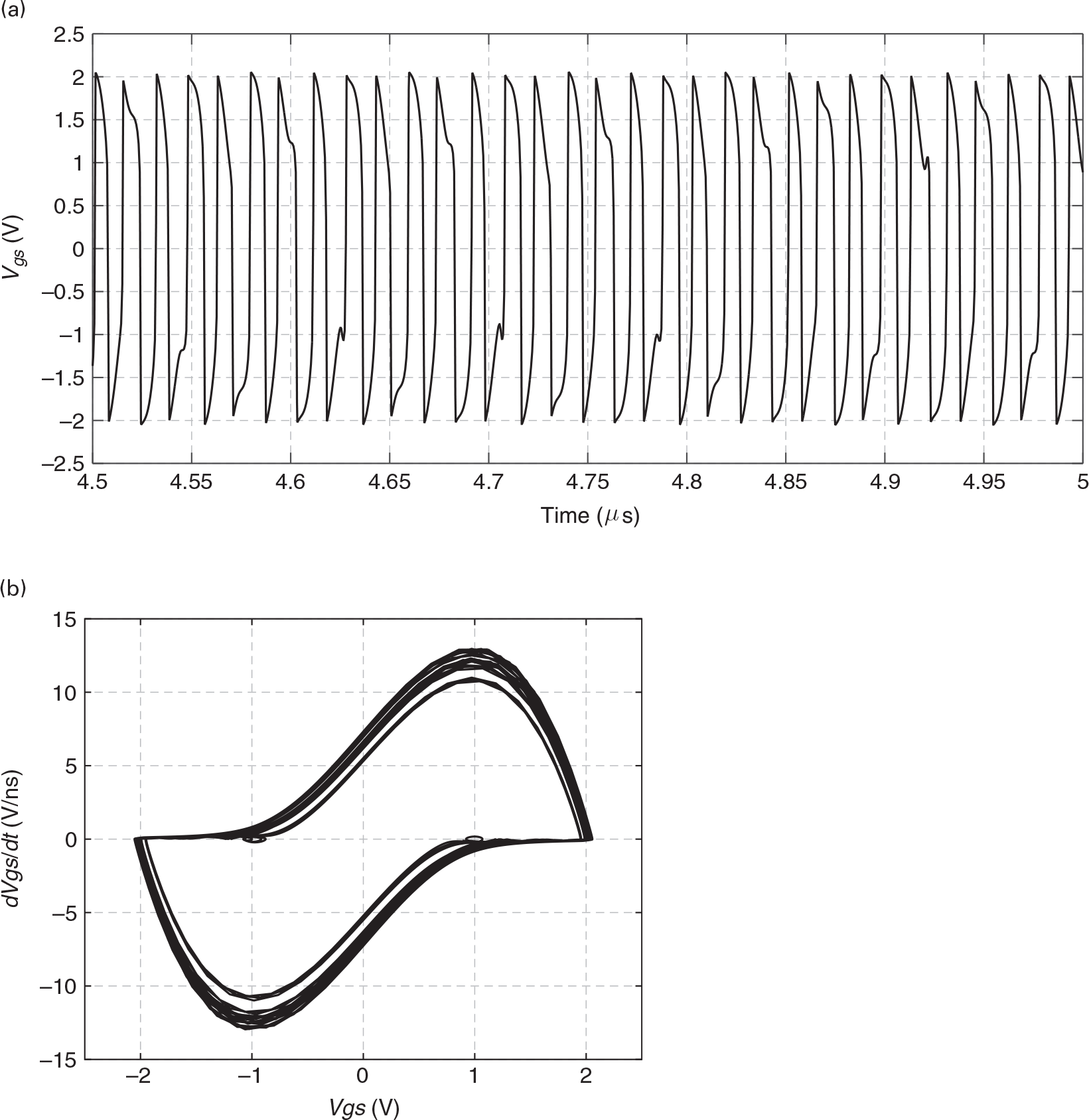
Figure 1.20 (a) vgs(t) voltage in time domain and (b) phase-portrait of the unstable amplifier in chaotic regime.
1.5 Example of a Static Transfer Nonlinearity
In the previous section, we illustrated the large variety of responses that can be expected from a nonlinear system. Now, we will try to systematize that, treating nonlinear systems according to their response types. That is what we will do in this and the next sections, starting from a static system to then evolve to a dynamic one. Because of the importance played by frequency-domain responses in RF and microwave electronics, we will start to study the system’s responses in the time domain and then observe their responses in the frequency domain.
1.5.1 The Polynomial Model
One of the simplest static nonlinear models we can think of is the polynomial because it can be interpreted as the natural extension of a static linear operator. Actually, the general Pth degree polynomial form of
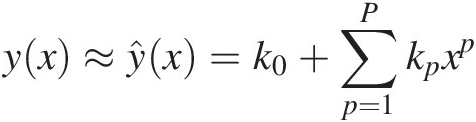 (1.28)
is a natural extension of the linear system model defined by ŷx=k1x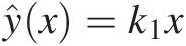 .
.
Moreover, polynomials have universal approximating properties, as they are known to approximate any analytic function, y(x), (one that is smooth, i.e., that is continuous and its derivatives with respect to the input are also continuous), as well as we want, in a certain input amplitude domain.
There is, however, something subtle hidden behind this apparent simplicity that we should point out. As happens to any other model, (1.28) does not define any particular model, but a model format, i.e., a mathematical formulation, or a family of models of our nonlinear static y(x)yx function, each one specified by a particular set of coefficients {k0, k1, k2, …, kp, …, kP}k0k1k2…kp…kP. To define a particular polynomial approximation, ŷx , for a particular function, y(x)yx, we need to find a procedure to identify, or extract, the polynomial model’s coefficients.
1.5.1.1 The Taylor Series Approximation
For example, we could start thinking of what would be the polynomial approximation that would minimize the error in the vicinity of a particular measured point [x0, y(x0)] and then let this error increase smoothly outside that region. Actually, this means that this polynomial approximation should be exact (provide null error) at this fixed point, x0, and thus it would have the following form:
 (1.29)
To identify these polynomial coefficients, we could start by realizing that differentiating (1.29) once with respect to x we obtain
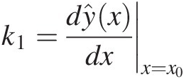 (1.30)
Then, performing successive differentiations we would be easily led to conclude that
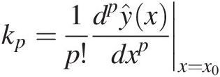 (1.31)
and that the polynomial approximation is the Taylor series given by
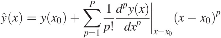 (1.32)
Note that the information that must be measured for extracting the P+1 coefficients of this polynomial is y(x0) plus the first P derivatives of y(x) in x0.
This Taylor series approximation is thus the best polynomial approximation in the vicinity of x0, or the best small-signal polynomial approximation in that vicinity. So, in our iD(vGS) function example, x0 can be regarded as the quiescent point VGS, k1 is the device’s transconductance in that quiescent point, and (x−x0) = (vGS−VGS) becomes the small-signal deviation [4], [16–17].
1.5.1.2 The Least Squares Approximation
Unfortunately, as this polynomial approximation directs all the attention to minimize the error in the vicinity of the fixed point, it cannot control the error outside that region, i.e., it may provide a good small-signal, or quasi-linear, approximation, but it will surely be very poor in making large-signal predictions. For these large-signal predictions, we have to find another coefficient extraction method that can take care of the y(x) function behavior in a wider region of its input and output domain than simply the vicinity of a particular fixed point.
For that, we will rely on one of the most attractive features of polynomial models, their linearity in the parameters. Although polynomial responses are obviously nonlinear to the input, they are linear-in-the-parameters, which means that, for example, the pth order polynomial response, kpxpkpxp, varies nonlinearly with xx, but linearly with its coefficient, or parameter, kpkp. And this is what allows the result in discrete time, y(nTs), of a polynomial approximation as (1.28) to be written as the following linear system of equations
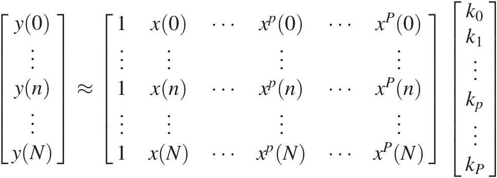 (1.33a)
or in matrix-vector form
and so to obtain the coefficients’ set as the solution of the following linear system of equations:
 (1.34a)
or
in which X−1X−1 stands for the inverse of the matrix XX, and y(0), …, y(N)y0,…,yN are the N + 1 = P + 1N+1=P+1 measured input and output data points [x(n), y(n)]xnyn.
Although, at this stage, we might think we have just said everything we could have said on polynomial model extraction, that is far from being the case. What we described was a procedure for finding just two specific polynomials. The first one, the Taylor series, focuses all its attention on one fixed point, providing a good small-signal prediction in that quiescent point, but discarding any specific details that may exist outside the vicinity of that point. The second passes through N + 1 = P + 1N+1=P+1 measured points, distributed in a wider input domain, but still pays no attention to how the approximation behaves in between these measured data points. Actually, specifying that the polynomial approximation should pass exactly through each of the measured points may not be a good policy, simply because of a fundamental practical reason: you may not be approximating the function, but a corrupted version of it due to the inevitable measurement errors. Fortunately, none of these can be said to be the polynomial approximation of y(x)yx in the defined input domain, but one of many possible polynomial approximations of that function in that domain. Different sets of coefficients result in different polynomial approximations, and to say that one is better than the other we should first establish an error criterion.
The most widely accepted criterion is the normalized mean square error (NMSE), a metric of the normalized (to the output average power) distance between the actual response y(n)yn and the approximated one, ŷn ,
,
 (1.35)
in which n, or nTs, is again the index of the discrete time samples. Please note that, expressed this way, the model is not approximating the function but its response to a particular input, x(nTs)xnTs, which indicates that you may obtain a different set of coefficients, for a different realization of the input. Actually, this is true for any model or model extraction procedure: we never approximate the system operator, but its observable behavior under a certain excitation or group of excitations, which reveals the importance of the excitation selection. Therefore, to find a model that takes care of the error outside the previously mentioned P + 1 observation points, we have to give it information on the function behavior between these points. In other words, we have to increase the number of excitation points.
At this point it should be obvious that to extract P + 1 coefficients we need, at least, P + 1 realizations, or N + 1 = P + 1 time samples of the input, x(n)xn, and the output, y(n)yn. However, nothing prohibits the use of more data points, and it should be intuitively clear that if we could provide more information about the system behavior (i.e., measured data) than the required minimum, it should not do any harm. On the contrary, it should even be better as we could, for example, compensate for the above referred measurement errors as finite resolution errors (or finite precision number representation) or random errors (due to instrumentation noise or other random fluctuations).
This is what is depicted in Figure 1.22, in which, beyond the ideal P + 1 [x(n), y(n)] point set, we have represented another P + 1 point set obtained from measurements, and thus corrupted by measurement errors. Please note that, although there is an ideal polynomial that passes exactly through the ideal P + 1 points (in this case P = 12), the polynomial that passes through the measured (P + 1 = 13) points is a different one.
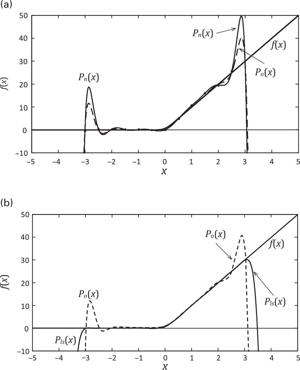
Figure 1.22 The polynomial approximation. (a) Po(x) is a 12’th degree polynomial that passes through 13 ideal, or error free, data points of f(x) in the [−3, +3] input domain, while Pn(x) is a similar polynomial but now extracted from 13 noisy measured data points. (b) Po(x) is the same 12’th degree polynomial of (a) extracted from error free data, while Pls(x) is another 12’th degree polynomial that approximates 200 error corrupted measured data points, in the least squares sense, in the same [−3, +3] input domain.
To overcome this modeling problem and move toward our objective of enlarging the approximation domain and providing an extraction method that is more resilient to data inaccuracies, we could think of obtaining a much richer data set to reduce the measurement error through some form of averaging. The question to be answered is: How can we use a larger number of measured data points, say 200 points, to extract the desired 12’th degree polynomial, taking advantage of the extra data points to correct the measurement errors? The answer to this question relies on augmenting the number of lines of (1.33). By doing that, we will relax the need of the 12’th degree polynomial to pass through all 200 points; we will only require that the model approximation passes close to the measured data in the minimum mean squared error sense of (1.35). That is, we will find the polynomial coefficient set that obeys
 (1.36)
Since it can be shown that there is only one minimum and no maximum, such a solution can be obtained by equating to zero the derivative of the error function with respect to the vector, k, of the polynomial coefficients, making
 (1.37)
This equation can be expressed as
 (1.38)
which can also be written as
 (1.39)
or, in matrix form, as
which can be solved for k through
in which XT stands for the transpose matrix of X. This minimum squared error solution is also depicted in our polynomial approximation example of 1.22.
There is an interpretation of this derivation that is worth discussing. It arises when we realize that the left-hand side of (1.39) and (1.40), XTy, is the cross-correlation at zero of the measured output, y(n), with each of the polynomial model kernels, xp(n), while their right-hand side is the product of the cross-correlation of all model kernel responses with themselves, the so-called regression matrix (XTX) times the model coefficients, k [18]. Indeed, the discrete cross-correlation between two time functions x(n) and y(n) is calculated by
 (1.42)
If the excitation were selected so that each model kernel response was independent, or uncorrelated, of all the others, i.e., if
 (1.43)
except when p1 = p2, we would say that the model kernels’ responses to that particular excitation were orthogonal, and the regression matrix (XTX) would be a diagonal matrix composed by the responses’ auto-correlations at zero. In that case, the coefficients were simply the cross-correlation of the output to its corresponding model kernel, normalized by the power (auto-correlation at zero) of the corresponding model kernel response. Hence, each of the model coefficients, kp, would be a measure of “how much” of its corresponding model kernel, xp(n), is in the observed output, y(n), in a similar way as the coefficients of the Fourier series of a signal constitute a metric of “how much” of the corresponding harmonic components are in that signal1.
In the opposite extreme case, i.e., when the excitation is poorly selected so that two or more kernels cannot be independently exposed, the regression matrix has a nearly zero determinant, the linear system of equations of (1.40) is then said to be ill-conditioned, and the coefficients cannot be correctly extracted.
1.5.2 Time-Domain Response of a Static Transfer Nonlinearity
The calculation of the response of our (static) polynomial to a general excitation in time domain is a trivial task. Since a static system responds to an excitation in an instantaneous way (i.e., it only reacts to the excitation at the present time), the system response at any arbitrary instant t0t0, y(t0)yt0, can be given by the algebraic computation of the model of our system at that instant t0t0, y(t0) = S[x(t0)]yt0=Sxt0. Thus, the response to a general excitation x(t)xt can be given by the successive application of this rule for each time instant: y(t) = S[x(t)] = k0 + k1x(t) + k2x2(t) + k3x3(t) + …yt=Sxt=k0+k1xt+k2x2t+k3x3t+….
1.5.3 Frequency-Domain Response of a Static Transfer Nonlinearity
To express the response of our polynomial static nonlinearity in the frequency domain, we will start again by stating that x(n) should be expressed as the discrete Fourier series
 (1.44)
where Xq is the abbreviated form of X(qω), which we will then substitute in (1.28) to obtain
 (1.45)
This time-domain response can then be rewritten to give
 (1.46)
in which Yq, or Y(qω), stands again for the qω frequency component of y(t) and constitute the desired frequency-domain response model. A close look into the second order response of (1.46) reveals that the Fourier component at, for example, the second harmonic, +2ω, results from the products of the component pairs at [−(Q−2),Q], [−(Q−3),(Q−1)], …, [−1,3], [0,2], [1,1], [2,0], [3,−1], …, [Q,−(Q−2)]. In general, as expressed in (1.46), the result at qω results from all possible summations of terms arising from products of the components at any q1ω and (q–q1)ω, i.e., (1.46) is a discrete convolution. As a matter of fact, originating, in the time domain, from the product of x(t) by itself, in the frequency domain it should correspond to a convolution of X(ω) by itself. Consequently, the p’th order term of (1.46), which arises from the time-domain product of x(t) by itself p times, results in the convolution of X(ω) by itself p times.
What we have just found leads us to an important property of static nonlinear systems, which we will find many other times during the course of our study. Because the response at the time sample n, y(n), only depends on the excitation of that time sample, x(n), i.e., it is a local operation, it can be calculated point by point, regardless of the excitation at any other time instant. However, that same static nonlinear function becomes a nonlocal operation, when computed in the frequency domain, since the response at each qω depends, in general, of the excitation’s input frequency content at all frequencies.
The property we have just described is a consequence of the fact that the Fourier transform of a local function of time (frequency), such as a product, has its support spread throughout all frequencies (times), since it is converted in a convolution. Actually, we had already seen a nonlocal operation in time, which was the convolution that arose as the response of dynamic linear systems. And, in that case, it was the frequency-domain response that was local, as it was given by the product of the Fourier-transform of the impulse response function by the Fourier transform of the input stimulus.
These important conclusions are summarized in Figure 1.23.

Figure 1.23 Local and nonlocal responses in time and frequency domains: (a) depicts the time and frequency mappings found in linear dynamic systems, which are nonlocal in time but local in frequency, while (b) illustrates the local in time and nonlocal in frequency mappings of nonlinear static systems.
1.6 Example of a Dynamic Transfer Nonlinearity
Now that we have already addressed the example of a static transfer nonlinearity, we can pass to a dynamic one. For that, we will review the linear case and explain how we can generalize it to the nonlinear domain. Similarly to what we have done with the static case, we will first obtain the time-domain response of our dynamic system and then move to derive its frequency-domain counterpart.
1.6.1 Time-Domain Response of a Dynamic Transfer Nonlinearity
When, in Section 1.2, we were reviewing the time-domain response of a linear time-invariant dynamic system to an input x(t), we concluded that it should have the form of a convolution of this stimulus x(t) with the impulse response function h(t). If the system were assumed stable, causal, and of finite memory, the impulse response function would start at t = 0 and last up to some memory span t = T. In the discrete time nTs, we would say that, if h(mTs) is the response to a unity impulse centered at nTs, and the input can be expressed as a combination of successive past impulses appearing at nTs, (n−1)Ts, …, (n−M)Ts, or simply, n, (n−1), …, (n−M), then the system response at nTs, y(n), can be expressed as the summation, or linear combination, of h(0)x(n), h(1)x(n−1), …, h(M)x(n−M), which constitutes the discrete convolution, as illustrated in Figure 1.24:
 (1.47)
Therefore, in linear systems, we can assume that the response to a summation of one unity impulse at nTs, x(n), and another at (n−1)Ts, x(n−1), is the summation of their responses, as if they were applied separately, as shown in Figure 1.24. In nonlinear systems that is not the case; superposition no longer applies, and (1.47) becomes invalid. In fact, we can even question the usefulness of having x(t) expanded as a summation of some predefined basis function as the Dirac delta function.
Nevertheless, we need to start from something to be able to proceed, and so we will keep this expansion of the input stimulus. Hence, we will assume that, beyond the linear response, the system responds to a pair of impulses, say x(n) and x(n−1), with some unknown response that depends on the magnitude of the two impulses and on their relative location. Unfortunately, this still involves such a high level of generality that impedes any progress. However, we can try to move another small step forward if we assume that this two-impulse response is similar to the one that we could expect from a polynomial, i.e., something like k2x2(n), 2k2x(n)x(n−1) and k2x2(n−1). Unfortunately, our intuition tells us that this cannot yet be right as we know that, if the system has memory, its response to the two impulses must depend on the relative position of the two impulses and present a tail in time. So, we should consider different coefficients and different contributions for any of the two different impulse times.
For example, if the two impulses were both present at the same time, we should have something like
 (1.48)
But, if the two impulses appeared at different instants in time, we should now have the following more general bidimensional form
 (1.49)
in which h2(m1,m2) plays a similar role as the linear impulse response h(m), but now for the second order response. If h(m), or h1(m), is the linear, or first order, impulse response function, h2(m1,m2) is the system’s nonlinear second order impulse response function.
So, the generalization of (1.47) from linear to nonlinear systems and the generalization of (1.28) from a static polynomial to one with memory must be given by [18]
 (1.50)
Expressed in continuous time, each of these discrete multidimensional convolutions becomes a continuous convolution in a similar way as the first order one of (1.6) turned into (1.7), and the summations of (1.50) become multidimensional integrals (see, e.g., [19]).
This model plays an important role in nonlinear dynamic systems since it is the simplest one can conceive to represent, simultaneously, nonlinear and dynamic behavior. Furthermore, its derivation can give important hints on the inherent complexity necessary to model these nonlinear dynamic devices. Nevertheless, it should be noted that, although (1.28) is a universal approximator of static analytic functions, (1.50) is restricted to dynamic operators that, beyond being analytic, must also be causal and stable and possess finite memory. In fact, the summations of (1.50) have support on only the present and the past time (the summation indexes m can only take positive integer values) (causality), the model cannot mimic any unstable behavior as it does not incorporate feedback (stability), and the present output does not depend on the inputs that appeared in an infinitely remote past, but are limited to x(n−MTs) (finite memory).
Similarly to what we said about the static polynomial of (1.28), this dynamic polynomial is only a general form and its complete specification depends on the particular way the coefficients are determined.
If the coefficients of (1.50) are selected as multidimensional partial derivatives in a predefined fixed point, [x0, h0 = y(x0)], (1.50) becomes a Taylor series with memory, also known as the Volterra series [19]. The coefficients that define the first order impulse response function of (1.47) and (1.50) constitute the linear dynamic response in the vicinity of the quiescent point, and all the other higher order coefficients acquire a similar role. If, on the other hand, an approximation in the minimum mean square error sense is desired, then the coefficients must be determined through a generalization of what was already discussed for the static case. Indeed, since (1.50) can be expressed as

 (1.51a)
or
then the coefficients that minimize the mean squared error must be given by
Before closing this subject, it is convenient to discuss two issues. The first one is related to an alternative interpretation of (1.50), while the second refers to the inclusion of feedback.
When studying linear system theory, we learned that a system like the one described by (1.47) was named a finite impulse response filter, FIR, and that (1.47) could be derived with a different, but obviously equivalent, reasoning. In short, the idea was to say that if our system has a finite memory, its response, y(n), must be given as a function of the present input, x(n), and all the past samples up to the memory span, x(n−M):
Then, if we added that the system is linear, we were saying that this function f [.] was linear, which means that its output should be a linear combination of its inputs, i.e., a summation of all of its M + 1 inputs, each one multiplied by a coefficient, and the result was the one of (1.47).
If we now take this idea and want to generalize it to a nonlinear system, we would say that, if f [.] was nonlinear, (1.53) would now represent some kind of nonlinear finite impulse response filter, or nonlinear FIR filter. And if, beyond that, we would say that we would approximate the (M + 1)-to-1 multidimensional function f [.] by a polynomial, (1.50) would become the linear combination of (1.47) for the first order response, the second order combination of (1.49) for the second order response, and so on, ending up with the complete response of (1.50). So, the hp(m1, …, mp)hpm1…mp parameters can either be interpreted as groups of coefficients that constitute the system’s discrete p’th order nonlinear impulse response functions or seen separately as the coefficients of a P’th order (M + 1)-to-1 multidimensional polynomial approximation of our nonlinear FIR filter.
Actually, this alternative interpretation of (1.50) can even allow us to generalize the introduced model of our nonlinear dynamic system in two different directions.
One way to generalize this is to say that the polynomial form of (1.50) is only a particular approximation of the desired multidimensional function f [.] and other possibilities could be tried. For example, if f [.] was approximated by a multidimensional table in which the delayed inputs x(n−m) are the indexing data and the table content is some interpolation of the measured y(n) response, we would have a time-delayed look-up table, TD-LUT, model. As another alternative, we could approximate f [.] by an artificial neural network [20] of the form
 (1.54)
in which bo, the output bias, wo,p, the output weights, bi,p, the input biases, and wi,m,p, the input weights, are fitting coefficients and fa[.], the activation function, is some appropriate nonlinear function, typically a sigmoidal function like the hyperbolic tangent, fa(x) = tanh (x)fax=tanhx, or a radial-basis function like the Gaussian, fa(x) = exp (−x2)fax=exp−x2. This structure, named the time-delay artificial neural network, TD-ANN, is depicted in Figure 1.25.

Figure 1.25 The time delay artificial neural network model which can be seen as a generalization of the polynomial FIR filter.
Another more elaborate way to generalize (1.50) is to say that the delayed versions of the input are simply one of many possible alternatives of including memory. In general, we could say that a nonlinear FIR model could be represented as a 1-to-(M + 1) linear dynamic filter bank followed by a (M + 1)-to-1 nonlinear static function as shown in Figure 1.26, the so-called Wiener Canonic Model [19].

Figure 1.26 Canonic Wiener Model as a generalization of the nonlinear polynomial FIR filter. It is composed of a 1-to-(M + 1) linear dynamic filter bank followed by a (M + 1)-to-1 static, or memoryless, nonlinear function.
Another, even more general way to express the response of a nonlinear dynamic system, would be to lift the restriction that the system should be stable and of finite memory. For that, we again recall what we learned from linear systems in that beyond the linear feedforward FIR model, we could also have a recursive, or feedback, infinite impulse response, IIR, filter of the form
so that (1.47) would become
 (1.56)
and (1.50) could be generalized to be
 (1.57)
Please note that this model now involves feedback and so it can be used to model unstable or even autonomous systems. In fact, feeding the input from the past outputs and starting from a nonzero initial output state, the output can either decrease in time toward zero or tend to any steady-state constant, increase or decrease without bound, or tend to a steady-state periodic or chaotic oscillatory behavior, mimicking the wide range of different behaviors we noted in Section 1.4. Unfortunately, this new capability may become a disadvantage when, due to imperfections of the model, we realize that we were using an unstable model to represent a stable system.
Another issue worth noting is that (1.52) can still be used to extract such a model as long as the y, X, and h matrices are augmented accordingly. In particular, beyond the input information, X now also includes past output data. However, it is also true that if the feedforward FIR model already involves a huge number of coefficients, this number is further increased in the IIR model of (1.57).
Finally, we would like to make a short note to say that it is not difficult to conceive a structure similar to the Canonic Wiener Model, but now with feedback, and so to imagine corresponding generalizations of the above mentioned TD-LUT and TD-ANN models.
1.6.2 Frequency-Domain Response of a Dynamic Transfer Nonlinearity
Similarly to what we did to obtain the frequency-domain response of first the linear dynamic and then the nonlinear static systems, we will start by stating again the decomposition of the input in the Fourier series of (1.44). Then substituting it in the nonlinear FIR filter of (1.50), we get
 (1.58)
Grouping the summations on the indexes mp and n, separately, and defining the multidimensional frequency-domain transfer function, Hp(q1ω, …, qpω)Hpq1ω…qpω or Hp(q1, …, qp)Hpq1…qp, as the multidimensional Fourier transform of the p’th order nonlinear impulse response function
 (1.59)
we get
 (1.60)
From this expression, we can now derive the desired Fourier coefficients of the y(n) time-domain response, Y(qω) or Yq, as
 (1.61)
which is again a series of frequency-domain convolutions, but now weighted by the nonlinear transfer functions Hp(q1, …, qp)Hpq1…qp. Actually, this expression is a generalization of the one obtained for the static case, Eq. (1.46). Since a static system has no memory, its response is independent of frequency, and therefore Hp(q1, …, qp)Hpq1…qp is a constant, kp, which can be written outside the summation. This independence of the Hp(q1, …, qp)Hpq1…qp transfer functions on frequency is the mathematical statement of the fact that the system is static or memoryless as, in that case, its response cannot depend on the excitation past but only on the present excitation, which implies that hp(m1, …, mp)hpm1…mp must be zero except when all m1, …, mpm1,…,mp are zero. This means that hp(m1, …, mp)hpm1…mp is a multidimensional impulse and so its Fourier transform Hp(q1, …, qp)Hpq1…qp must be constant.
1.7 Summary
The objective of this first chapter was to give the reader a detailed introduction to nonlinear systems.
We started by showing that although nonlinearity is essential to wireless communications and present in the majority of RF and microwave circuits, it is usually not given the necessary attention because we lack the elegant and simple analytical tools we were accustomed to use in linear circuits.
In an attempt to show the relationship between what is known from the linear systems and what is studied for the first time about the nonlinear systems, we tried to show how nonlinear systems, i.e., their characteristics and their mathematical modeling tools, can be understood as a generalization of linear systems. However, we hope we also conveyed the message that because linearity is a very restrictive concept that can be condensed into a simple mathematical relation – the superposition principle – this generalization to nonlinear systems is much more complex in terms of both the type of responses and required mathematical analyses than one might expect. On the other hand, it is exactly this complexity of behaviors, and their importance, that make nonlinear circuits an exciting topic and an attractive area for research and practice.
1.8 Exercises
Exercise 1.1 A voltage amplifier with offset is a circuit that presents an open-circuit output voltage, vo(t), that can be related to its input voltage vi(t) as vo(t) = Avvi(t) + Voffsetvot=Avvit+Voffset. Using (1.1) and (1.2), prove that such an amplifier is nonlinear, even if its input–output graphic representation is a straight line.
Exercise 1.2 What could be done to convert our voltage amplifier of Exercise 1.1 into a linear system?
Hint: Interpret the offset, VoffsetVoffset, as the response to a second independent variable, or stimulus.
Exercise 1.4 Prove again that the ideal amplitude modulator of Exercise 1.3 must be nonlinear, but now using the result of Section 1.2, which stated that the response of any linear system (dynamic or static) to a sinusoid is another sinusoid of the same frequency.
Exercise 1.5 Show that the ideal amplitude modulator, which, as seen in Exercise 1.3, must inherently be a nonlinear system of two inputs (the modulation envelope and the carrier) and one output (the resulting modulated signal) can be seen as a linear time-variant system of one single input (the modulation envelope) and one output (the same resulting modulated signal).
Exercise 1.6 Prove that the sinusoidal oscillator model of Eq. (1.15) indeed represents a linear system.
References
 Findit@CUHK Library | Google Scholar
 Findit@CUHK Library | Google Scholar
 Findit@CUHK Library | Google Scholar
 Findit@CUHK Library | Google Scholar
 Findit@CUHK Library | Google Scholar
 Findit@CUHK Library | Google Scholar
 Findit@CUHK Library | Google Scholar
 Findit@CUHK Library | Google Scholar
 Findit@CUHK Library | Google Scholar
 Findit@CUHK Library | Google Scholar
 Findit@CUHK Library | Google Scholar
 Findit@CUHK Library | Google Scholar
 Findit@CUHK Library | Google Scholar
 Findit@CUHK Library | Google Scholar
 Findit@CUHK Library | Google Scholar
 Findit@CUHK Library | Google Scholar
 Findit@CUHK Library | Google Scholar
 Findit@CUHK Library | Google Scholar
 Findit@CUHK Library | Google Scholar
 Findit@CUHK Library | Google Scholar