The main goal of this chapter is to review the various nonlinear simulation techniques available for RF and microwave circuit analysis, and to present the basic operation and properties of those techniques. Although this is not intended to be a course on nonlinear analysis or simulation, which is far beyond the scope of this book, we believe it is still important for the reader to have a basic idea of how these simulation tools function. This way, he or she can select the most appropriate technique for their particular task and be aware of its limitations.
Although mathematical details will be kept to a minimum, they can still intimidate many microwave engineers. If this is the case, do not worry, stick to the qualitative explanations and the physical interpretations provided to describe the equations. Ultimately, this is more important than the mathematical derivations themselves.
Before we move on to discuss the details of each of the simulation techniques, it is convenient to first state a set of rules common to all of them. So, we start by defining what is meant by circuit or system simulation.
As explained in Chapter 1, the concept of system can be used in its most general form to represent either circuit elements, circuits, or complete RF systems. Therefore, we will use the notion of system whenever we want to achieve this level of generality, and we will adopt the designation of circuit element, component, circuit, or RF system otherwise.
Nowadays, circuit or RF system simulation is a process in which the behavior of a real circuit or RF system is mimicked, solving, in a digital computer, the equations that – we believe – describe the signal excitation and govern the physical operation of that circuit. Hence, the success of simulation should be evaluated comparing the real circuit or RF system behavior with the one predicted by the simulator. The simulation accuracy depends on both the adopted equations and the numerical techniques used to solve them. The set of equations that represent the behavior of each element constitutes the model of the element. The set of equations that describe how these are connected (the circuit or RF system topology) defines the model of the system. The numerical techniques, or numerical methods, used to solve these equations are known as the numerical solvers.
Contrary to linear systems, most nonlinear systems found in practice are described by complex nonlinear equations that do not have any closed form solution. Hence, there is no way to get a general understanding of the system’s behavior and we have to rely on partial views of its response to a few particular excitations. This is the underlying reason why simulation plays a much more important role in nonlinear circuit or RF system design than in its linear counterpart.
Currently, the discipline of mathematics on numerical methods is so advanced that the accuracy limitation of modern circuit simulators resides almost entirely on the models’ accuracy. But, since the circuit’s equations are often derived from nodal analysis (a statement of the universal law of charge conservation), we would not be exaggerating if we said that circuit simulation accuracy limitations must be solely attributed to the circuit components models, or to a possible misuse of the simulator (for example, expecting it to do something for which it was not intended).
Because it is the users who select the simulator, and most of the time, it is their responsibility to provide the simulator with the appropriate models, it is essential that they have, at least, a basic understanding of what the simulator does, so that they can a priori build a rough estimate of the simulation result. Otherwise, the entire simulation effort can be reduced to a frustrating “garbage in, garbage out.”
Actually, the main objective of this book is to provide the knowledge to the RF/microwave engineer that prevents falling into any of these traps. The present chapter aims at a correct use of the simulator, while the next four address the components’ models.
This chapter on simulation is organized in four major sections. Section 2.1 deals with the mathematical representation, or model, of signals and systems. Section 2.2 treats time-domain simulation tools for aperiodic and periodic regimes. Hence, its main focus is the transient analysis of SPICE-like simulators. Although Section 2.2 already addresses the steady-state periodic regime in the time-domain, via the so-called periodic steady-state, or PSS, algorithm, this is the core of the harmonic-balance, HB, frequency-domain technique of Section 2.3. Finally, Section 2.4 describes a group of algorithms especially devoted to analyze circuits and telecommunication systems excited by modulated RF carriers. From these, special attention is paid to the envelope-transient harmonic-balance, ETHB, a mixed-domain – time and frequency – simulation tool.
2.1 Mathematical Representation of Signals and Systems
As said above, simulation tools comprise the mathematical representation – equations or models – of the system whose behavior is to be predicted, and the numerical solvers for these equations. Therefore, this subsection is intended to introduce general forms for these representations. For that, we will consider the wireless transmitter depicted in Figure 2.1.
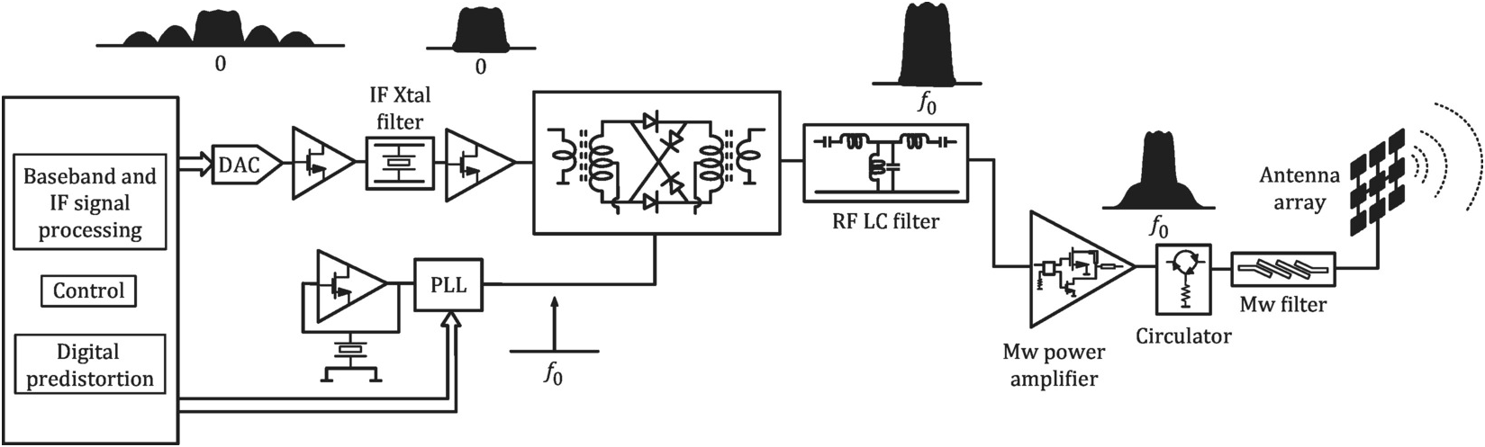
Figure 2.1 The block diagram of a wireless transmitter used to illustrate the disparate nature of circuits and signals dealt with by RF circuit designers.
2.1.1 Representation of Circuits and Systems
In the wireless transmitter example in Figure 2.1 we can recognize a very heterogeneous set of circuits such as digital signal-processing and control, mixed digital-analog, analog IF or baseband, and RF. Considering only this latter subset, we can note circuits that operate in an autonomous way, like the local oscillator, and ones that are driven, and thus present a forced behavior. In addition, we may also divide them into circuits solely composed of lumped elements (like ideal resistors, capacitors, inductors, and controlled sources) or into ones that include distributed elements (such as transmission lines, microstrip discontinuities, waveguides, etc.).
2.1.1.1 Circuits of Lumped Elements
As seen in Chapter 1, the response of dynamic circuits or systems cannot be given as a function of solely the instantaneous input, but depends also on the input past, stored as the circuit’s state. For example, in lumped circuits, i.e., circuits composed of only lumped elements, their state comprises the electric charge stored in the capacitors and the magnetic flux stored in the inductors, the so-called system’s state-variables or the state-vector. Assuming that these capacitor charges and inductor fluxes are memoryless functions of the corresponding voltages and currents (the quasi-static assumption in which accumulated charges, fluxes, or currents are assumed to be instantaneous functions of the applied fields), the state-equation is thus the mathematical rule that describes how the state-vector evolves in time. It is an ordinary differential equation, ODE, in time that expresses the time-rate of change of the state-vector, i.e., its derivative, with respect to time, as a function of the present state and excitation:
 (2.1)
(2.1)where s(t) is state-vector, x(t) is the vector of inputs, or excitation-vector, (independent current and voltage sources) and f[s(t), x(t)]fstxt is a set of functions, each one derived from applying Kirchhoff’s currents law, KCL, to the nodes, and voltages law, KVL, to the branches.
With this state-equation, one can calculate the trajectory of the state-vector over time, s(t). Then, it is easy to compute the output-vector, y(t), i.e., the set of observable currents, voltages, or any algebraic operation on these (such as power, for example) from the following output-equation:
For an illustrative example of this state- and corresponding output-equations, let us use the circuit of Figure 2.2. The application of Kirchhoff currents law to the input and output nodes, leads to
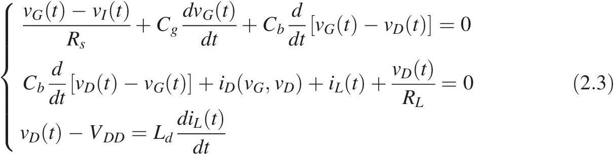 (2.3)
(2.3)which can be rewritten as
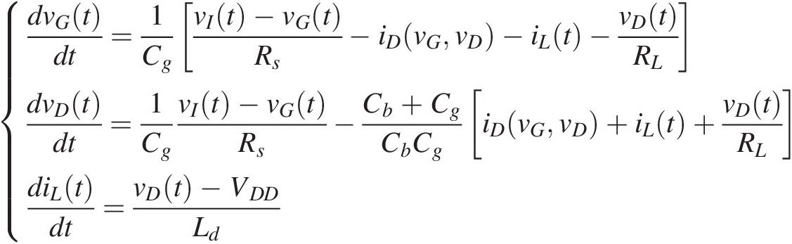 (2.4)
(2.4)Defining now s1(t) ≡ vG(t), s2(t) ≡ vD(t), s3(t) ≡ iL(t), x1(t) ≡ vI(t)s1t≡vGt,s2t≡vDt,s3t≡iLt,x1t≡vIt and x2(t) ≡ VDDx2t≡VDD allows us to express these nodal equations in the canonical state-equation form of (2.1) as
 (2.5)
(2.5)where N = 3, M = 2N=3,M=2 and
 (2.6)
(2.6)Assuming that the desired observable is the output voltage, vO(t)vOt, the canonical output equation can be obtained following a similar procedure, defining y(t) ≡ vO(t) = vD(t) = s2(t)yt≡vOt=vDt=s2t
which, in this case, is simply y(t) = s2(t)yt=s2t.
Figure 2.2 Simplified FET amplifier circuit (a) and its equivalent circuit (b) intended to illustrate the analysis’s algorithms. vI(t) = VGG + vS(t) where vS(t) is the excitation, VGG = 3 V, VDD = 10 V, Rs = 50 Ω, Cg = 50 pF, Cb = 4.4 pF, Ld = 120 nH, and RL = 6.6 Ω. The MOSFET has a transconductance of gm = 10 A/V, a threshold voltage of VT = 3 V, and a knee voltage of VK = 1 V.
Because this system is a third order one, its behavior is completely described by a three-dimensional state-vector, i.e., involving three state-variables. So, as explained in Section 1.4.4, its phase-portrait should be represented in a volume whose axis are s1, s2, and s3, or vG, vD, and iL, as is shown in Figure 2.3. Please note that the state-variables correspond to the expected circuit’s three independent energy storing elements: s1(t) ≡ vG(t)s1t≡vGt is a measure of the accumulated charge (electric field) in the input capacitor Cg, s2(t) ≡ vD(t)s2t≡vDt is needed to build vGD(t) = vG(t) − vD(t) = s1(t) − s2(t)vGDt=vGt−vDt=s1t−s2t, a measure of the accumulated charge in the feedback capacitor Cb, and s3(t) ≡ iL(t)s3t≡iLt stands for the accumulated magnetic flux in the output drain inductor Ld.
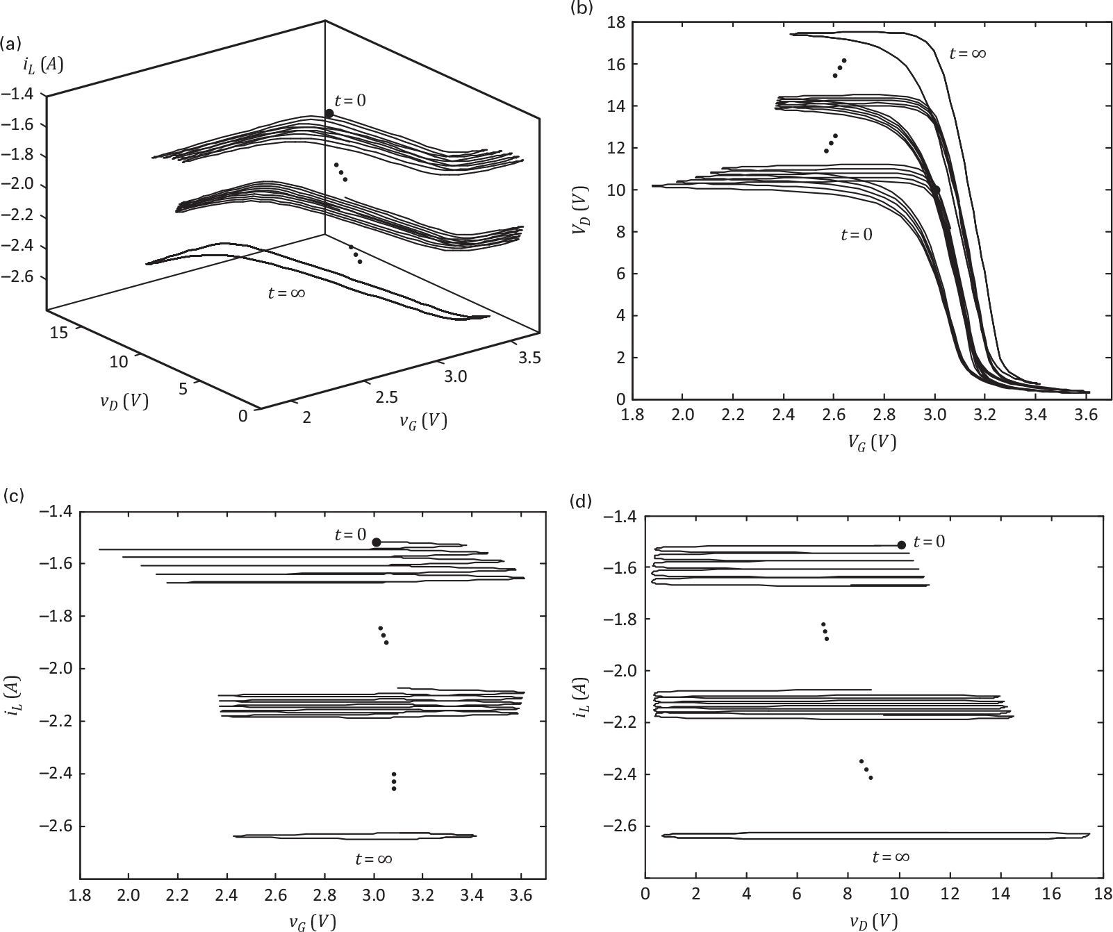
Figure 2.3 (a) Illustrative trajectory of the three-dimensional system state, [x y z] ≡ [vG vD iL], of our example circuit. (b) Projection of the 3D state-space trajectory onto the [vG vD] plane. (c) Projection of the 3D state-space trajectory onto the [vG iL] plane. (d) Projection of the 3D state-space trajectory onto the [vD iL] plane.
Although the phase-portrait is a parametric curve in which the evolving parameter is time, it does not allow a direct observation of the trajectory of each of the state-variables over time. In fact, a graph like Figure 2.3 (a) cannot tell us when the system is more active or, on the contrary, when it is almost latent. Such a study would require separate graphs of s1(t), s2(t) or s3(t) versus time as is exemplified in Figure 2.4 for s1(t) and s2(t).
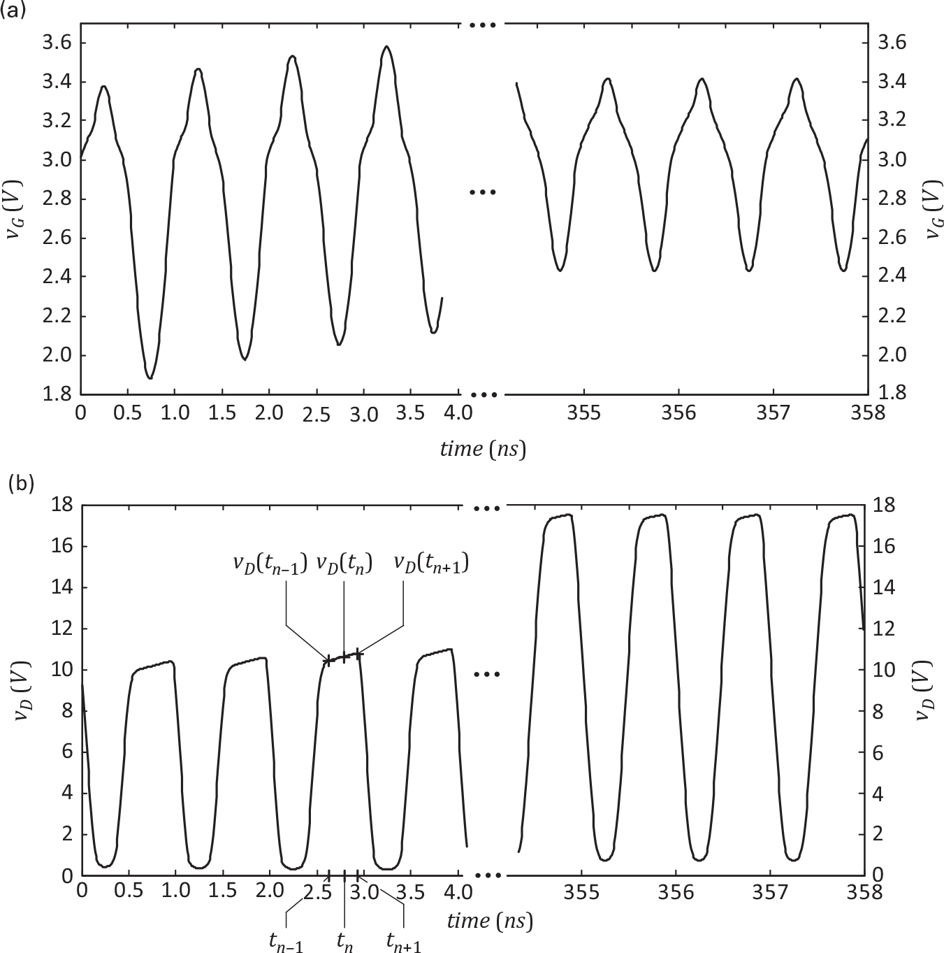
Figure 2.4 Time evolution of two of the system’s state-variables over time. (a) s1(t) = vG (t) and (b) s2(t) = vD(t).
2.1.1.2 Circuits with Distributed Elements
Contrary to circuits that include only lumped elements, circuits or systems that involve distributed components, such as transmission lines or other distributed electromagnetic multi-ports, cannot be described as ODEs in time, requiring a description in both time and space. That is the case of the power divider/combiner, the circulator or the output microwave filter of Figure 2.1, and of the transmission line of Figure 2.5. As an example, the transmission line is described by the following partial differential equations, PDEs, in time, t, and space, x.
 (2.8)
(2.8)where i(x, t)ixt and v(x, t)vxt are the distributed current and voltage along the line and R, L, C, and G, stand for the usual line’s distributed resistance, inductance, capacitance, and conductance per unit length, respectively.
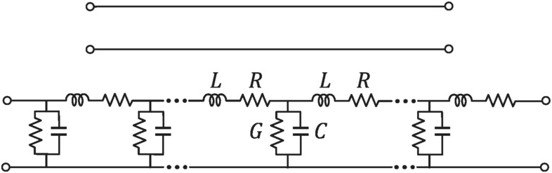
Please note that, because all time-domain circuit simulators are programmed to solve ODEs, they require that the circuit be represented by the state- and output-equations of (2.1) and (2.2). Consequently, a lumped representation is needed for distributed components. Such lumped representation is usually given in the form of an approximate equivalent circuit, obtained from the frequency-domain behavior observed at the device ports, which mimics the operation of the original multiport [1]. However, alternative behavioral representations, such as the one based on the impulse response function and subsequent convolution with the component’s excitation, are also possible [2].
It should be emphasized that these are behavioral representations, not real equivalent circuits, as distributed elements do not have a true lumped representation. For example, even our uniform transmission line of Figure 2.5 would need an infinite number of elementary lumped RLCG sections. Therefore, if one is willing to simulate such a circuit in the time domain, he or she should be aware that he is not simulating the actual circuit but another one that, hopefully, produces a similar result. For example, if the extracted “equivalent” circuit is not guaranteed to obey certain properties, such as passivity [3], one may end up with nonconvergence results or erroneous solutions such as a nonphysical (and so impossible) oscillatory response from an original circuit composed of only passive components.
2.1.2 Representation of Signals
As far as the signals are concerned, we could group them into baseband – or slowly evolving – information signals, fast-varying RF carriers, and modulated signals, in which the first two are combined. Furthermore, as shown in the spectra included in Figure 2.1, we could also note that, contrary to the RF carriers, which are periodic and thus narrowband, baseband signals are wideband (that span through many octaves or decades) and are necessarily aperiodic, as they carry information (nonrepeatable, by definition). Therefore, while the periodic RF carrier can be represented in either the time or frequency domains, baseband signals must be necessarily treated in the time domain since the discrete Fourier series assumes periodicity in both time and frequency. Actually, because we will be using a digital computer, i.e., a machine with a finite number of states, it will necessarily impose a discrete, or sampled and of confined nature, description of any time- or frequency-domain entities. This means that if you want to represent, in the frequency domain, a certain continuous-time signal, extending from, say, 0 to T seconds, what you will get is the frequency-domain representation of another discrete and periodic signal, of period T, which extends from –∞ to +∞, and whose sampling frequency, fs, is determined by the computer time resolution. Such a signal has a discrete and periodic spectrum whose frequency resolution is Δf = 1/T and whose period is fs. Conversely, any continuous spectrum signal will be treated as one of discrete spectrum, which has a periodic time-domain representation. In addition, any Fourier conversion between these two domains will necessarily be executed via the discrete Fourier transform, DFT, or its fast version, the FFT, in case the number of time and frequency points is a multiple of two.
2.2 Time-Domain Circuit Analysis
This section deals with circuit analysis techniques that operate in the time domain, such as SPICE or SPICE-like transient simulators [4], [5], and the ones known for calculating the periodic steady-state in the time domain. These simulators assume that the excitation-vector is known for the period of time where the response is desired and that the circuit is represented by the state- and output-equations of (2.1) and (2.2). In addition, it is assumed that the response is desired as a waveform in the time-domain.
2.2.1 Time-Step Integration Engines
Time-step integration is used in all SPICE-like transient simulators [4], [5] but also in many system simulators [6–8]. Since it aims at the evolution of the circuit in time, it can be seen as the most “natural” circuit analysis technique because it closely follows the conceptual interpretation we make of the circuit operation. Actually, assuming one starts from a known excitation, x(t), discretized in a number of appropriate time-points, x(tn), and an also known, initial state, s(t0), one can easily compute the response at all future time samples, s(tn), from the discretization of the state-equation. This discretization reflects the knowledge that the derivative of the state at the time, tn, is the limit when the time-step length, hn, tends to zero, of the ratio [s(tn + 1) − s(tn)]/hnstn+1−stn/hn. Therefore, the state-equation (2.1) can be approximated by the following difference equation
 (2.9)
(2.9)which allows the calculation of all s(tn) using the following recursive scheme known as the forward Euler method [9]
in a time-step by time-step basis. It is this time-step integration of the state-equation that constitutes the root of the name of this family of methods.
Alternatively, we could have also approximated the state derivative at tn by
 (2.11)
which would then lead to the alternative recursive scheme of
which is known as the backward Euler method.
Despite the obvious similarities between (2.10) and (2.12) (originated in their common genesis), they correspond to very distinct numerical methods. First of all, (2.10) gives the next state, s(tn+1), in an explicit way, since everything in its right-hand side is a priori known. On the contrary, (2.12) has an implicit formulation since the next state s(tn+1) depends on the known s(tn) and x(tn+1), but also on itself. Hence, s(tn+1) can be obtained through simple and fast algebraic operations from (2.10), while the solution of (2.12) demands for an iterative nonlinear solver, for which it is usually formulated as
Actually, (2.13) can be solved using, e.g., a gradient method like the Newton-Raphson iteration [10].
A Brief Note on the Newton-Raphson Iteration
The Newton-Raphson iteration plays such an important role in nonlinear circuit simulation that we will outline it here. Based on a first order Taylor series approximation, it finds the zero of a nonlinear function, or vector of functions, through the solution of a successively approximated linear system of equations. In the present case, the vector of functions whose zero is to be calculated is φ[s(tn + 1)] ≡ s(tn + 1) − s(tn) − hnf[s(tn + 1), x(tn + 1)]φstn+1≡stn+1−stn−hnfstn+1xtn+1 and so its first-order (linear) Taylor approximation in the vicinity of a certain predetermined estimate, s(tn + 1)istn+1i, becomes
where Jφ[s(tn + 1)i]Jφstn+1i is the Jacobian matrix of φ[s(tn + 1)]φstn+1 whose element of row m and column l is calculated by
 (2.15)
i.e., it is the derivative of the m’th component of the vector of functions φ[s(tn + 1)]φstn+1 with respect to the l’th component of the state-vector s(tn + 1)stn+1, evaluated at the previous estimate s(tn + 1)istn+1i.
Since (2.14) is now a linear system in the unknown s(tn + 1)i + 1stn+1i+1, we can get a (hopefully) closer estimate of the desired zero by the following iteration:
This is graphically illustrated in Figure 2.6 (a) for the simplest one-dimensional case. Please note that, if φ[s(tn + 1)]φstn+1 were linear, its Jacobian matrix would be constant, i.e., independent of s(tn + 1)istn+1i, and the Newton-Raphson algorithm would converge in only one iteration. In general, the Newton-Raphson method is faster in presence of mildly nonlinear problems and slower – i.e., it needs more iterations – when dealing with strongly nonlinear problems (higher curvature in the function of Figure 2.6). Furthermore, it requires an initial estimate of the solution, and converges if the function φ[s(tn + 1)]φstn+1 is well behaved, i.e., if its Jacobian matrix has no points of zero determinant. In fact, if s(tn + 1)istn+1i is a point in the state-space in which the determinant of the Jacobian is zero, or close to zero, the next estimate will suffer a big jump, possibly to a point very far from the desired solution φ[s(tn + 1)] = 0φstn+1=0, even if it were already close to it at s(tn + 1)istn+1i. As illustrated now in Figure 2.6 (b), the Newton-Raphson iteration of (2.16) may diverge from the target solution even when it is already quite close to it. Alternatively, since in the vicinity of a zero determinant Jφ[s(tn + 1)i]Jφstn+1i changes sign, the iteration may be stalled, endlessly jumping from two distinct points as depicted in Figure 2.6 (c). In this case, (2.16) does not diverge, but it cannot also converge to the solution.

Figure 2.6 Graphical illustration of the Newton-Raphson iteration in the simplest one-dimensional case. (a) Normal convergence of the Newton-Raphson iteration. (b) When the function of which we want to calculate the zero, φ(s)φs, has a zero in its derivative (the Jacobian), the iteration may diverge from the desired solution. (c) Situation in which the iteration does not either diverge or converge but is kept wandering around the vicinity of a zero derivative point.
Unfortunately, the simplicity of (2.10) has a high price in numerical stability. Since it is a predictive method, its associated error tends to build up very rapidly, a problem that must be obviated by reducing the time-step, and thus increasing the overall simulation time. In practice, this increase in simulation time and the potential numerical instability are so significant, when compared to (2.12), that (2.10) is hardly ever used in practical circuit simulators.
Actually, (2.10) and (2.12) do not constitute the only way that we could have used to integrate the state-equation. They are just examples of a zero-order method in which the derivative is assumed constant during the time-step interval. For example, if a first-order integration (known as the trapezoidal integration rule) would have been used, we would obtain [8]
 (2.17)
In general, the time-step integration scheme is formulated as
 (2.18)
from which the 4th-order Runge-Kutta method [8] is one of its most popular implementations (see Exercise 2.1).
Finally, it should be added that there is no need to keep the time-step, hn, constant. In fact, all modern time-domain simulators use dynamic time-steps, measuring the variation in time of s(t). Larger time-steps are used when s(t) is slowly varying, while smaller ones are adopted in zones of fast change of state. This way, a good compromise between accuracy and computation time is obtained.
Example 2.2 The Time-Step Integration Formulation
As an example of time-step integration, the trapezoidal rule discretization of our circuit example described by (2.5) and (2.6) would lead to
 (2.19)
where the three f(tn)ftn were defined in (2.6).
For each time step, tn, (2.19) is a nonlinear system of three equations in three unknowns, s1(tn+1), s2(tn+1) and s3(tn+1), which can be solved by the Newton-Raphson iteration of (2.16) making
 (2.20a)
or in a compacted form
 (2.20b)
and

 (2.21a)
or
 (2.21b)
where I stands for the identity matrix, and gm(t) and gds(t) are, respectively, the FET’s transcoductance and output conductance, defined by gmt=∂iDvGvD∂vGvGt,vDt and gdst=∂iDvGvD∂vDvGt,vDt
 .
.
Figures 2.3 and 2.4 depict the results of the simulation of (2.16) for an excitation of vI(t) = VGG + vS(t) = 3 + 20 cos (2πfct)vIt=VGG+vSt=3+20cos2πfct, fc = 1 GHz, and with s1(0) = 3.0 V, s2(0) = 10.0 V and s3(0) = −10/6.6 A initial conditions. This time-step integration used the trapezoidal rule of (2.19) and a fixed time step of h = 1/(100fc).
If the frequency-domain response representation is desired, as is quite common in RF and microwave circuit analysis and design, then a DFT must be performed on the time-domain response, which requires that the signal is uniformly sampled and periodic.
Unfortunately, and as we have seen, simulation speed determines the use of dynamic time-steps, which produces a non-uniformly sampled response. So, either one forces the simulator to use a fixed time-step, e.g., using the simulator’s time-step ceiling option – turning the time-domain simulation highly inefficient – or relies on the hidden interpolation and resampling functions operated before the DFT is applied, which are not error free – turning the frequency-domain representation potentially inaccurate.
If the signal is not periodic, then the DFT will make it periodic, with a period equal to the simulated time, producing an error that is visible as spectral leakage [10], i.e., in which the energy of individual spectral lines is distributed onto (leaks to) their vicinity. This error is caused by the time-domain signal discontinuities that may exist in the beginning and end points of the constructed periodic signal and is illustrated in Figure 2.7. It is particularly harmful in distortion analysis where the distortion components may be totally immersed in the spectral leakage error. Hence, it is quite common to adopt measures to mitigate spectral leakage, increasing the simulation time (in order to reduce the relative weight of these discontinuities in the overall signal) or to simply eliminate these discontinuities, forcing the output signal to start and end in the same zero value – y(0) = y(T) = 0 – multiplying y(t) by an appropriate window function [10].

Figure 2.7 Illustrative example of the spectral leakage generated when an aperiodic time-domain function is (discrete) Fourier transformed to the frequency domain. Please note the spectral leakage manifested as erroneous spectral power around the desired signal and its mitigation by windowing. In this example, VdTω is the frequency-domain representation of five periods of the result of our transient simulation, vD(t), collected between 50 ns and 55 ns, while VdHω
 is the corresponding signal passed through a Hanning window [10]. The dotted spectrum, VdSω
 , is the same five periods but now collected after the steady-state was reached, i.e., collected between 380 ns and 385 ns.
This lack of periodicity of the output signal can be due to the nature of the problem at hand. For example, a two-tone signal of f1 and f2 is only periodic if its central frequency fc = (f1 + f2)/2 is a multiple of its frequency separation Δf = f2 − f1. But it may also be due to the presence of the transient response. In such a case, it is necessary to truncate the signal to its last few periods. This process is usually quite frustrating when simulating RF circuits since the length of this annoying transient response can be many orders of magnitude higher than the length of the desired period, or of a few periods. Indeed, the length of these long transients is usually determined by the time-constants associated to the large dc decoupling capacitors and RF chokes of bias networks.
Therefore, this transient time-domain simulation of microwave and RF circuits tends to be either inefficient, inaccurate, or both, which motivated the development of analysis techniques specifically devoted to calculate the periodic steady-state.
2.2.2 Periodic Steady-State Analysis in the Time-Domain
Although one might think that the integration of the transient response is unavoidable, as it corresponds to the way the real circuit behaves, that is not necessarily the case. To understand why, let us recall the previously discussed problem that consists in determining the response of a forced system to a periodic excitation of period T. To guarantee that this problem is solvable, let us also consider that the steady-state response is, indeed, periodic, of the same period T of the excitation.
Obviously, the complete response starts with the aperiodic transient, which is then followed by the periodic steady-state. This transient is naturally governed by the system, the excitation and the assumed initial conditions, or initial state, while the periodic steady-state is only dependent on the system and the excitation (in fact, its period is solely determined by the excitation). Therefore, different initial states lead to distinct transient responses, but always to the same steady-state. Actually, a close observation of Figures 2.3 and 2.4 indicates that different initial states may lead to transients of very different length, depending on whether we start from an initial state that is close, or very far, from the final cyclic orbit that describes the periodic steady-state. In fact, the notion of state tells us that all states of that cyclic orbit keep the system in the same orbit, i.e., lead to a transient response of zero length or, in other words, a response without transient.
Example 2.3 A Time-Step Integration Simulation that Does Not Exhibit a Transient
Although the mere existence of a transient simulation without a transient may sound absurd, you can convince yourself that this can indeed be true by running the following example. Pick up any lumped-element circuit you know, which, being excited by a periodic stimulus, produces a periodic steady-state response. Perform a normal transient simulation using a SPICE-like circuit simulator for a time that is sufficiently long to let the circuit reach its periodic steady-state. You will naturally see a transient response followed by the periodic steady-state. Analyze this steady-state response, observing and recording the values of all state-variables, for example all capacitor voltages and inductor currents, at the beginning (arbitrary) of one period of the excitation. Now, run the same transient simulation but use the simulator option that allows you to set the initial values of all energy-storage elements to the values previously recorded (use all precision digits the simulator provides). You can run the transient simulator for a much smaller time-span as you will see that the response is completely periodic, i.e., that there is no transient response.
We actually performed this experiment in our circuit example, starting with the same initial conditions and excitation used for our previous transient simulation, i.e. vG(0) = 3.0 V, vD(0) = 10.0 V, iL(0) = −10/6.6 A and vI(t) = 3 + 20 cos (2π109t)vIt=3+20cos2π109t, measured these variables at t = 384 ns, and then used these values [vG(384 ns) = 3.118026263640600 V, vD(0) = 11.183192073318860 V and iL(0) = −2.625494710083924 A] as the new initial conditions. As expected, the simulator response went directly to the steady-state response of Figures 2.3 and 2.4 without any transient.
By the way, this example leads us to this very curious question: which were, after all, the energy-storage initial conditions used by default by the simulator in the first run? And how did it select them? You will find a response to these questions in the next section.
Now that we are convinced that our problem of bypassing the transient response may have a solution, it becomes restricted to find a way to determine these appropriate initial states (see Exercise 2.2). There are, at least, three known techniques to do that.
The first method we can imagine to determine the proper initial states (i.e., the ones that are already contained in the cyclic orbit) was already discussed. Indeed, although the time-step integration starts from an initial state that may be very far from the desired one, the state it reaches after one period, is closer. Then, this new updated state is inherently used as the initial state for the time-step integration of the second period, from which a new update is found, in a process that we know is convergent to the desired proper initial state. Our problem is that this process is usually too slow due to the large dc decoupling bias network capacitors and RF chokes. In an attempt to speed up the transient calculation, a simple dc analysis (in which all capacitors and inductors are treated as open or short circuits, respectively) is performed prior to any transient simulation. Then, the dc open circuit voltages across the capacitors and the short-circuit currents across the inductors are used as the initial conditions of the corresponding voltages and currents in the actual transient simulation, unless other initial conditions are imposed by the user. These dc values constitute, therefore, the default initial state that the simulator uses. When these dc quiescent values are already very close to the actual dc bias values, as is the case of all linear or quasi-linear circuits, such as small-signal or class A power amplifiers, the transient response is short and this method of finding the default initial conditions can be very effective. Otherwise, i.e., in case strongly nonlinear circuits such as class C amplifiers or rectifiers are to be simulated, these default values are still very far from the actual bias point and a large transient response subsists.
The second and third methods find the proper initial condition using a completely different strategy: they change the nature of the numerical problem.
2.2.2.1 Initial-Value and Boundary-Value Problems
Up to now, we have considered that our circuit analysis could be formulated as an initial-value problem, i.e., a problem defined by setting initial boundary conditions (the initial state) and a rule for the time evolution of the other internal time-steps (the state-equation). No boundary conditions are defined at the end of the simulation time; as we know, this simulation time can be arbitrarily set by the user. When we are willing to determine the periodic steady-state, and we know a priori that the steady-state period is the period of the excitation, we can also define a final boundary condition and reformulate the analysis as a boundary-value problem. In this case the initial state, the internal rule, and the final state are all a priori defined. Well, rigorously speaking, what is defined is the internal rule and an equality constraint for the initial and the final states: s(t0 + T) = s(t0).
2.2.2.2 Finite-Differences in Time-Domain
Having this boundary-value problem in mind, the second method is known as the finite-differences in time-domain and is directly formulated from the discretization of the state-equation and the periodic boundary condition s(t0 + T) = s(t0). Using again a zero-order backward Euler discretization in N + 1 time-samples, we can define the following (incomplete) system (for each state-variable or each circuit node) of N equations in N + 1 unknowns
 (2.22)
which, augmented by the boundary equation s(tN) = s(t0), constitutes a (now complete) system of N + 1 equations in N + 1 unknowns that can be readily solved through a N + 1-dimensional Newton-Raphson iteration scheme.
2.2.2.3 Shooting Method
The third alternative to find the proper initial condition that leads to the desired steady-state is known as the shooting or periodic steady-state, PSS, method. Conceptually, it can be described as a trial-and-error process in which we start by simulating the circuit for one period with some initial state guess; for example, the one given by an a priori dc analysis, s(t0)1st01. In our circuit example, this attempt would lead to the first set of trajectories depicted in the phase-space plots of Figure 2.8, in which s(tN)1≠s(t0)1stN1≠st01, indicating, as expected, that we failed the periodic steady-state. By slightly changing the tested initial condition by some Δs(t0)Δst0, say s(t0)2 = s(t0)1 + Δs(t0)st02=st01+Δst0, we can try the alternative attempt identified as the second set of trajectories of Figure 2.8. Although this one led to another failure, since s(tN)2stN2 is still different from s(t0)2st02, it may provide us an idea of the sensitivity of the final condition to the initial condition, Δs(tN)/Δs(t0)ΔstN/Δst0, which we then may use to direct our search for better trial s(t0)3st03, s(t0)3st03, …, s(t0)Kst0K, until the desired steady-state is achieved, i.e., in which s(tN)K = s(t0)KstNK=st0K.

Figure 2.8 Illustration of the shooting-Newton method of our circuit example excited by vI(t) = 3 + 20 cos (2π109t)vIt=3+20cos2π109t, where all the required five Newton iterations are shown. As done for the previous transient analysis, we started from the initial conditions derived from dc analysis, vG(0) = 3.0 V, vD(0) = 10.0 V and iL(0) = −10/6.6 A, and ended up on vG(0) = 3.118026121336410 V, vD(0) = 11.183189430567937 V and iL(0) = −2.625492967125298 A.
Actually, using a first order Taylor series approximation of the desired null error, s(tN) − s(t0) = 0stN−st0=0, we may write [11], [12]:
 (2.23)
which leads to the following Newton-Raphson iteration:
 (2.24)
known as the shooting-Newton PSS method. It should be noted that this sensitivity matrix, ΔstNΔst0 , can be evaluated along the time-step integration of the period, using the chain differentiation rule as
 (2.25a)
where
 (2.25b)
directly from the time-step integration formula of (2.18).
Example 2.4 The Shooting-Newton Formulation
In our circuit example, where we used the trapezoidal integration rule, this recurrent formula can be derived from (2.20) and (2.21) by noting that, if φ[s(tn + 1)] = 0φstn+1=0, then
 (2.26)
and so


and finally
 (2.27)
Although the shooting-Newton PSS is based on an iterative process to find the appropriate initial state, it is, by far, much more efficient than the other two preceding methods for at least three reasons [12]. The first one is that, while (2.22) attempts to solve a N + 1-dimensional problem at once, (2.24) solves it resolving N + 1 one-dimensional problems, one at a time. The second is that the sensitivity, or the Jacobian, of (2.24) can be computed along with the transient simulation. Finally, the third is that although the circuit may be strongly nonlinear, the dependence of the final condition on the initial condition seems to be only mildly nonlinear in most practical problems, so that the Newton-Raphson solver converges in just a few iteration steps. For example, as is illustrated in the phase-state plots of Figure 2.8, the application of the shooting-Newton algorithm to our circuit example needed only five iterations to reach the desired periodic steady-state, even if we started from the same initial condition used for the transient analysis.
These properties make the PSS the technique of choice for efficiently computing the periodic steady-state regimes in time-domain of RF and microwave circuits. However, the inexistence of time-domain models for many RF and microwave components (mostly passive components such as filters and distributed elements, which are usually described by scattering parameter matrices) and the fact that, many times, RF/microwave designers operate on stimuli and responses represented as spectra, make frequency-domain methods, such as the harmonic-balance, the most widely used simulation techniques in almost all RF/microwave circuit designs.
2.3 Frequency-Domain Circuit Analysis
As you may still recall from basic linear analysis, and from what was discussed in Chapter 1, frequency-domain methods are particularly useful to study the periodic steady-state for two different reasons.
The first of these reasons concerns the computational efficiency, because a sinusoid, which should be represented in the time domain by several time samples, requires only two real values (or a single complex value) when represented in the frequency domain. Indeed, knowing that the response of a linear system to a sinusoid is also a sinusoid of the same frequency, the sinusoidal response becomes completely described by its amplitude and phase. Furthermore, if the system’s excitation and response are not pure sines but a superposition of sines that are harmonically related, then we still need two real values for each represented harmonic. Actually, the harmonic zero, i.e., dc, requires only one value, as its phase is undefined.
The second reason for the paramount role played by frequency-domain techniques, is a consequence of the fact that the time-derivative of a complex exponential of time (or of a sinusoid, as they are related by the Euler’s formula) is still the same complex exponential of time multiplied by a constant:
 (2.28)
This converts an ordinary linear differential equation into a much simpler algebraic equation. In fact, assuming that both the excitation and the state are periodic of period T = 2π/ω0T=2π/ω0, then, x(t) and s(t) can be represented by the following Fourier series
 (2.29)
 (2.30)
which, substituted in the state-equation of (2.1)
 (2.31)
in which A1 and A2 are the two matrices that uniquely identify our linear system, results in
 (2.32)
or
an algebraic linear system of equations in the vector Sk, the Fourier components of s(t). Exercise 2.3 deals with an example of this linear formulation.
2.3.1 Harmonic-Balance Engines
The application of the Fourier series representation to the analysis of nonlinear systems assumes that, for a broad set of systems (namely the ones that are stable and of fading memory [13]), their steady-state response to a sinusoid, or to a periodic excitation, of period T, is still a periodic function of the same period. However, as we already know from the harmonic generation property of nonlinear systems, this does not mean that the frequency content of the response is the same of the input. It simply means that it is located on the same frequency grid, ωk = kω0ωk=kω0. In general, the harmonic content of the output is richer than the one of the input, although there is, at least, one counter-intuitive example of this: linearization by pre- or post-distortion, in which a nonlinear function and its inverse are cascaded. Please note that this assumption of periodicity of the steady-state response of our system to a periodic excitation (in the same frequency grid) is a very strong one. If it fails (for example, if the system is chaotic or is unstable, oscillating in a frequency that falls outside the original frequency grid) frequency-domain techniques may not converge to any solution or, worse, may converge to wrong solutions without any warning.
The extension of the frequency-domain analysis of linear systems to nonlinear ones is known as the harmonic-balance, HB, since it tries to find an equilibrium between the Fourier components that describe the currents and voltages in all circuit nodes or branches. It is quite easy to formulate, although, as we will see, not so easy to solve. To formulate it, we simply state again the Fourier expansions of (2.29) and (2.30) and substitute them in the state-equation (2.1), to obtain
 (2.34)
Within the stable and fading memory system restriction, we do know that the right-hand side of (2.34) will be periodic of fundamental frequency ω0, and thus admits the following Fourier expansion:
 (2.35)
in which S(ω) and X(ω) stand for the Fourier components vectors of s(t) and x(t), respectively. Substituting (2.35) in (2.34) results in
 (2.36)
which would not be of much use if it weren’t for the orthogonality property of the Fourier series. In fact, since the complex exponentials of the summations of (2.36) are orthogonal – which means that no component of ejk1ω0tejk1ω0t can contribute to ejk2ω0tejk2ω0t unless k1 = k2 − (2.36) can actually be unfolded as a (nonlinear) system of 2K + 1 equations (for each state-variable or circuit node), of the form
in 2K + 1 unknowns (the Sk). Written in vector-matrix form, (2.37) can be expressed as
in which jΩ is a diagonal matrix whose diagonal values are the jkω0.
Please note that since there is no known method to compute the nonlinear mapping [S(ω),X(ω)]→F(ω) for any general function f[s(t),x(t)] or F[S(ω),X(ω)] directly in the frequency domain, one has to rely on the time-domain calculation, f[s(t),x(t)], converting first S(ω) and X(ω) to the time domain, and then converting the resulting f(t) = f[s(t),x(t)] back to the frequency domain. These frequency-time-frequency domain transforms constitute a heavy burden to the HB algorithm, which has motivated the quest for a pure frequency-domain alternative, nowadays known as spectral-balance [14].
The idea is to express f[s(t),x(t)] with only arithmetic operations, for which the frequency-domain mapping is known. For example, if f[s(t),x(t)] is expressed as a polynomial – which is nothing else but a summation of products – the time-domain addition corresponds to a frequency-domain addition, while the time-domain product corresponds to a frequency-domain spectral convolution (which can be efficiently implemented as the product of a Toplitz matrix by a vector [15]). Actually, this same idea can be extended to more powerful rational-function approximators (i.e., ratios of polynomials) since the time-domain division corresponds to a frequency-domain deconvolution, which is implemented as the product of the inverse of the Toplitz matrix just referred by a vector [15]. Although the spectral-balance has not seen the same widespread implementation of the traditional harmonic-balance, it is still interesting as a pure frequency-domain nonlinear simulation technique.
To solve the nonlinear system of equations of (2.38), we can again make use of the multidimensional Newton-Raphson algorithm, for which we need to rewrite (2.38) in its canonical form as
Then, the Newton-Raphson iteration would be
in which JF[S(ω), X(ω)] stands for the Jacobian matrix of the frequency-domain function F[S(ω), X(ω)].
Unfortunately, the previous phrase may be misunderstood because of its apparent simplicity. In fact, if we said that we did not know any direct way to compute F[S(ω), X(ω)] in the frequency domain, we certainly do not know of any way to compute its Jacobian either. However, this Jacobian plays such an important role in nonlinear RF circuit analysis that we cannot avoid digging into its calculation. Therefore, to retain the essential, without being distracted by accessory numerical details, let us imagine we have a simple one-dimensional function of a one-dimensional state-variable: f(t) = f[s(t)] or F(ω) = F[S(ω)]:
 (2.41)
The row m and column l of the wanted Jacobian matrix, JF[S(ω)]ml, is thus the partial derivative of the m’th Fourier component of F(ω), Fm, with respect to the l’th Fourier component of S(ω), Sl:
 (2.42)
Now, as the order of the derivative and the integral can be interchanged, using the derivative chain rule that allows us to write
 (2.43)
and thus
 (2.44)
which is the (m − l)’th Fourier component of the derivative of f(s) with respect to s, g(s).
A physical interpretation of this result can be given if we consider that, for example, f(s) represents a FET’s drain-source current dependence on vGS, iDS[vGS(t)]. In this case, g[s(t)] is the FET’s transconductance and so (2.44) stands for the (m − l)’th Fourier component of the time-variant transconductance, gm(t) = gm[vGS(t)], in the large-signal operating point, LSOP, [vGS(t), iDS(t)]. It constitutes, thus, the frequency-domain representation of the device operation linearized in the vicinity of its LSOP, an extension of the linear gain, or transfer function, when the device is no longer biased with a dc quiescent point, but with one that is time-variant and periodic.
Therefore, this Jacobian is the frequency-domain time-variant transfer function of a mixer whose LSOP is determined by the local-oscillator (maybe with also a dc bias), known in the mixer design context as the conversion matrix [16], [17]. Beyond this, the position of the poles of the Jacobian’s determinant provide valuable information on the large-signal stability of the circuit, in much the same way as the poles of the frequency-domain gain of a time-invariant linear amplifier – biased at a dc quiescent point – determine its small-signal stability [18].
But, this Jacobian can represent much more than this if a convenient linear transformation of variables is performed in the circuits’ currents and voltages to build incident and scattered waves. If F[S(ω)] is defined so that it maps frequency-domain incident waves, A(ω) = S(ω), into their corresponding scattered waves, B(ω) = F[A(ω)], the Jacobian would correspond to a form of large-signal S-parameters (available in some commercial simulators), or, more rigorously, to the S and T parameters of the poly-harmonic distortion, PHD, or X-Parameters model, [19], [20] (as will be discussed in Chapter 4).
As always, an important issue that arises when one is trying to find the solution of a nonlinear equation like (2.39) with the Newton-Raphson iteration of (2.40), is the selection of an appropriate initial condition. From the various possible alternatives we might think of, there is one that usually gives good results. It assumes that most practical systems are mildly nonlinear, i.e., that their actual response is not substantially distinct from the one obtained if the circuit is considered linear in the vicinity of its quiescent point. Therefore, the simulator starts by determining this dc quiescent point, setting to zero all ac excitations, and then estimates an initial condition from the response of this linearized circuit.
If this does not work, i.e., if it is found that the Newton-Raphson iteration cannot converge to a solution, then the simulator reduces the excitation level down to a point where this linear or, quasi-linear, approximation holds. Having reached convergence for this reduced stimulus, it uses this response as the initial condition for another simulation of the same circuit, but now with a slightly higher excitation level. Then, this source-stepping process is repeated up to the excitation level originally desired.
Continuing to use our circuit example of Figure 2.2, with the same periodic stimulus vI(t) = 3 + 20 cos (2π109t)vIt=3+20cos2π109t, we will now solve it for its periodic steady-state using the harmonic-balance formulation. For that, we will use the time-domain state equations of (2.5) and (2.6) to identify F[S(ω), X(ω)]FSωXω in (2.39) and (2.40) as
 (2.45)
The application of the Newton-Raphson algorithm to (2.39) requires the construction of the Jacobian matrix JF[S(ω), X(ω)]. In this example of three state-variables, the Jacobian matrix will be a 3 × 3 block matrix whose elements are given by:
 (2.46)
in which Gm(ωm − l)Gmωm−l and Gds(ωm − l)Gdsωm−l are the (m − l)m−l frequency component of the device’s time-varying transconductance, gm(t)gmt, and output conductance, gds(t)gdst, respectively.
Figure 2.9 illustrates the evolution of the harmonic content of the output voltage of our example circuit, |Vd(kω0)| = |S3(kω0)|, during the Newton-Raphson solution of (2.40), while Figure 2.10 provides this same result but now seen in the time-domain, vD(t) = s3(t). Although the 3-D plot of Figure 2.9 presents only the first 15 harmonics plus dc, 50 harmonics were actually used in the simulation.

Figure 2.9 Illustration of the evolution of the first 15 harmonics, plus dc, of the amplitude spectrum of the output voltage, |Vd (kω0)| = |S3(kω0)|, during the first 50 Newton-Raphson iterations of the HB simulation of our example circuit. Note how the simulation starts by assuming that the output voltage is a sinusoid (at the fundamental frequency, k = 1) plus a dc value (k = 0), and then evolves to build its full harmonic content.

Figure 2.10 Illustration of the evolution of the time-domain steady-state harmonic-balance solution of vD(t) = s3(t), during the whole Newton-Raphson iterations. Note how the simulation starts by assuming that the output voltage is a sinusoid plus a dc value, and then evolves to build the correct waveform shape.
2.3.2 Piece-Wise Harmonic-Balance
In this section we introduce what became known as the piece-wise harmonic-balance method, to distinguish it from the nodal-based harmonic-balance analysis technique just described. In fact, in piece-wise HB we do not start by a nodal analysis – from which we derived the state-equation – but begin by separating all of the circuit’s current, charge, or flux nonlinear sources from the remainder of the linear subcircuit network, as is illustrated in Figure 2.11. Then, we only analyze the exposed circuit nodes, i.e., the ones to which nonlinear voltage-dependent charge or current sources are connected. Let us, for the sake of language simplicity, designate these exposed nodes as nonlinear nodes and linear nodes the ones contained in the linear subcircuit network. (Please note that, despite not mentioning them here, nonlinear current-dependent flux sources could have also been considered, although requiring a slightly different formulation).

Figure 2.11 Decomposition of a nonlinear microwave circuit into a subcircuit linear block to which the nonlinear voltage dependent current or charge sources are connected, as needed for the application of the piece-wise harmonic-balance technique.
In piece-wise HB, the variables we will determine are no longer the circuit’s state-variables, but only the voltages of these exposed nodes, V(ω). Because most microwave circuits have typically many more linear nodes than nonlinear ones, the dimension of V(ω) is usually much smaller than the one of S(ω), which constitutes an enormous computational advantage of the piece-wise HB with respect to its nodal-based counterpart. Now, we apply frequency-domain nodal analysis to these nonlinear nodes obtaining the following desired HB equation:
In (2.47), Inl[V(ω)]InlVω is the frequency-domain current vector representing the currents entering the nonlinear current sources, which, as before, must be evaluated in the time-domain as
 (2.48)
in the case of voltage-dependent nonlinear current sources, or as
 (2.49)
in the case of voltage-dependent nonlinear charge sources (nonlinear capacitances).
Il[V(ω)]IlVω stands for the current vector entering the linear subcircuit network, which is easily computed in the frequency domain by
in which Y(ω)Yω is the linear subcircuit network admittance matrix.
Finally, Ix[X(ω)]IxXω are the excitation currents that can be computed as
where the transfer matrix Ax(ω) can have either current gain or transadmittance gain entries, whether they refer to actual independent current source or independent voltage source excitations, respectively.
Please note that, while the nonlinear current sources, or the nonlinear subcircuit network, which is composed of only quasi-static elements, is treated in the time domain, the linear subcircuit, which contains all dynamic components (even the time derivatives of nonlinear charges), is directly treated in the frequency-domain.
This has an important advantage in terms of computational efficiency. Because static nonlinearities are treated in the time domain, they tend to require fast product relations, while they would need much more expensive convolution relations if dealt with in the frequency domain (as was seen when we discussed spectral-balance). On the other hand, linear dynamic elements necessitate convolution in the time domain, but only require product relations when treated in the frequency domain.
Finally, we should say that the piece-wise HB equation of (2.47) can be solved for the desired V(ω) vectors through the following Newton-Raphson iteration:
 (2.52)
For an application example of the piece-wise harmonic-balance method, see Exercise 2.4.
To summarize this description of the basics of the harmonic-balance – formulated in both its nodal and piece-wise form – Figure 2.12 depicts its algorithm in the form of a flowchart.

Figure 2.12 An illustrative flowchart of the harmonic-balance algorithm. Although this flowchart was formulated for HB applied to each node or state-variable, in its nodal form, it could be easily extended to be applied to only the nonlinear nodes, as is required for the piece-wise HB formulation.
2.3.3 Harmonic-Balance in Oscillator Analysis
Because oscillators are autonomous systems, i.e., systems in which there is no excitation, we would not think of them in the context of harmonic-balance. Indeed, the whole idea of HB is based on the a priori knowledge of the state-vector frequency set, something we are looking for in the oscillator analysis. However, a clever modification of HB allows it to be used for the determination of the steady-state regime of this kind of autonomous systems.
To understand how it works, let us consider the piece-wise HB formulation of (2.47), in which all but the dc components of the excitation vector, Ix[X(ω)]IxXω, are zero.
Please note that, dividing both sides of (2.53) evaluated at the fundamental by the corresponding (non-null) node voltage vector, would lead to
 (2.54)
which can be recognized as the Kurokawa oscillator condition [21]. So, using HB for oscillator analysis sums up to solve (2.53) for V(ω)Vω. The problem is that not only (2.53) is insufficient since it involves, at least, one more unknown than the available number of equations, as we already know one possible solution of it, that we do not want. In fact, if (2.47) was a determined system, (2.53) can no longer be because the oscillation base frequency ω0 is now also unknown. In addition, because Ix[X(ω)]IxXω is now zero, except for ω = kω0 = 0, one possible solution of (2.53) is the so-called trivial, or degenerate, nonoscillatory condition where all but the dc components of V(ω)Vω are zero. In the following, we will deal with these two problems separately.
The first of these problems can be solved noting that if it is true that because Ix[X(ω)]IxXω is now zero (except for ω = 0), and so there is no way to a priori know the basis of the frequency set, it also true that the phases of V(ω)Vω are undetermined, as we lost the phase reference. Well, rigorously speaking, only the phase of the fundamental is undetermined, as the phases of the harmonics are referenced to it. Actually, what is undetermined is the (arbitrary) starting time, t0, at which we define the periodic steady-state. In fact, since the system is time-invariant, it should be insensitive to any time shift, which means that if v(t) is a periodic solution of (2.53), than v(t − t0) should also be an identical solution of that same equation. In the frequency domain, this means that the phase of the fundamental frequency ϕ1 = −ω0t0 can be made arbitrary, while the phase of all the other higher-order harmonics are related to it as ϕk = −kω0t0 = −kϕ1. So, (2.53) is still a system of (2K + 1) equations in 2K + 1 unknown vectors: the vector of dc values V(0), K vectors of amplitudes of the fundamental and its harmonics, (K − 1) vectors of their phases (ϕ2…ϕK), plus the unknown frequency basis ω0. Therefore, it can be solved in much the same way as before, using, for example, the Newton-Raphson iteration, except that now there is a column vector in the Jacobian that is no longer calculated as ∂Fm/∂Sl but as ∂Fm/∂ω0.
The second problem consists in preventing the Newton-Raphson iteration on (2.53) to converge to the trivial, or degenerate, solution. As explained, this solution is the dc solution in which all but the 0’th harmonic components of V(ω)Vω are zero. One way to prevent this is to maximize the error for this particular trivial solution. This can be done normalizing the error of (2.53) by the root-mean-square voltage magnitude of non-dc V(ω)Vω:
 (2.55)
In commercial HB simulators, the adopted approach uses the so-called oscillator-probe. Its underlying idea is to analyze the oscillator, not as an autonomous system, but as a forced one. Hence, the user should select a particular node in which it is known that a small perturbation can significantly disturb the oscillator and apply a special source (the oscillator-probe) to it, as is represented in Figure 2.13.

Figure 2.13 Oscillator analysis via harmonic-balance of a nonautonomous system using the oscillator-probe.
Such an appropriate node is one that is in the oscillator feedback loop or close to the resonator. The oscillator-probe is a voltage source whose frequency ω0 is left as an optimization variable, and whose source impedance is infinite at all harmonics but the fundamental at which it is zero. So, this ZS(ω) behaves as a filter which is a short-circuit to the fundamental frequency, ω0, and a nonperturbing open-circuit to all the other harmonics kω0, where k≠1. Then, the oscillator analysis is based on finding the so-called nonperturbation condition, i.e., to determine ω0 and |VS| that make IS(ω0) = 0. Under this condition, the circuit behavior is the same whether it has the oscillator-probe attached to it or not. So, although this solution was found as the solution of a nonautonomous problem, it coincides with the solution of the original autonomous circuit.
2.3.4 Multitone Harmonic-Balance
The frequency-domain analysis technique presented above assumes a periodic regime for both the excitation and the state-vector, so that these quantities can be represented using the discrete Fourier transform. Unfortunately, there are a significant set of steady-state simulation problems that do not obey this restriction. Some of them, as chaotic systems, are so obviously aperiodic that we would not even dare to submit them to any frequency-domain analysis. Their spectra are continuous and so there is no point in trying to find the amplitude and phase of a set of finite discrete spectral lines. There are, however, other situations that are still aperiodic and thus cannot be treated using the DFT, but that can still be represented with a finite set of discrete spectral lines. They are the so-called multitone or almost-periodic, regimes. For example, consider a signal composed by the addition of two sinusoidal functions:
This excitation can be either periodic or aperiodic, depending on whether or not ω1 and ω2 are two harmonics of the same fundamental frequency. That is, if ω1 = k1ω0 and ω2 = k2ω0, then x(t) is periodic, and it is aperiodic if there is no ω0 that verifies both of these conditions. An equivalent way of stating x(t) periodicity is to stipulate that ω2/ω1 = k2/k1 is a rational number. Conversely, stating that x(t) is aperiodic is equivalent to stipulating that there are no two nonzero integer numbers, m1 and m2, that satisfy m1ω1 + m2ω2 = 0. Therefore, periodicity requires that ω1 and ω2 are commensurate (ω2/ω1 is a rational number), while we say that the aperiodic two-tone excitation is composed of two incommensurate frequencies (ω2/ω1 is an irrational number). In general, an excitation composed by a set of frequencies, ω1, …, ωKω1,…,ωK is aperiodic if, and only if, there is no set of nonzero integers that verify
In this context, we will restrict our multitone excitation to the case of incommensurate tones, as the other one can always be treated with the above described harmonic-balance algorithm for periodic regimes.
Let us then consider the two-tone excitation of (2.56), in which ω1 and ω2 are incommensurate. If it is true that neither x(t) nor s(t) can be expressed as a Fourier series, it is as well true that we may write x(t) as
 (2.58)
in which, Xk1, k2 = 0Xk1,k2=0 when |k1| + |k2|>1, for a pure two-tone excitation, and
 (2.59)
for s(t). In fact, experience tells us that the vast majority of nonlinear systems responds to a set of discrete spectral lines at ω1 and ω2, with a set of discrete lines located at all harmonics of ω1, all harmonics of ω2 and all possible mixing products of ω1 and ω2. So, although we cannot affirm that ωk = kω0, because the response is aperiodic, and so neither (2.58) nor (2.59) are Fourier series, we can state that these signals can still be expressed as a sum of discrete spectral lines whose location is a priori known.
Naturally, as it happened with periodic harmonic-balance, a certain spectrum truncation must be established. However, while in the periodic regime this was easily set in a single axis of frequencies as |k|ω0 ≤ Kω0, in the almost-periodic case, since we have two harmonic limits, K1 and K2, there is no unique obvious choice. On the contrary, there are at least two possibilities often used.
The first one establishes that |k1| ≤ K1 and that |k2| ≤ K2, in which K1 and K2 need not to be equal. For example, in mixer analysis, the highest harmonic order for the large-signal local oscillator must be significantly higher than the one used for the small RF signal. If the mixing products, k1ω1 + k2ω2, are represented as points in a plane defined by the orthogonal axes k1ω1 and k2ω2, then these conditions define a rectangular figure, or box, limited by K1ω1 and K2ω2. This is illustrated in Figure 2.14 for K1 = 2 and K2 = 3. That is the reason why this spectrum truncation scheme is known as box truncation.

Figure 2.14 Box truncation frequency set for |k1| ≤ 2 and |k2| ≤ 3 (35 mixing products). “X” indicates a used position of the bidimensional spectrum truncation.
The second truncation scheme derives from the practical knowledge that typical spectra tend to have smaller and smaller amplitudes when the order of nonlinearity is increased. This means that, if it can be accepted that the highest harmonic order for ω1 is, say, K1, and the maximum order for ω2 is K2, then a mixing product at K1ω1 + K2ω2 will certainly have negligible amplitude and box truncation may waste precious computational resources. So, the alternative is to consider a maximum harmonic order K and then state that |k1| + |k2| ≤ K. As illustrated in Figure 2.15, this condition leads to a diamond-shaped coverage of the frequency plane above described, which is the reason why it is known as the diamond truncation.

Figure 2.15 Diamond truncation frequency set for |k1| + |k2| ≤ 3 (25 mixing products). “X” indicates a used position of the bidimensional spectrum truncation.
After stating that the response to be found is given by (2.59), under an appropriate spectrum truncation scheme, multitone HB determines the coefficients SkSk, or Sk1, k2Sk1,k2, knowing that they can be related by
 (2.60)
In fact, there is no substantial difference between the multitone HB algorithm of (2.60) and its original periodic HB except that, now, we are impeded to evaluate the right-hand side of (2.60) in the time domain as we lack a mathematical tool to jump between time and frequency domains. Hence, what we will outline in the following are three possible alternatives to overcome this limitation.
2.3.4.1 Almost-Periodic Fourier Transform
The first multitone HB technique we are going to address takes advantage of the fact that, although neither x(t) nor s(t) are periodic, they can still be represented by a finite set of discrete spectral lines. They are, thus, named almost-periodic and its frequency-domain coefficients can be determined in a way that is very similar to the DFT and is named the almost-periodic Fourier transform, APFT [22]. To understand how, let us assume that, for simplicity, s(t) is a one-dimensional vector, s(t), defined in a discrete time grid of t = nTs. If it can be expressed as (2.59) we may write
 (2.61a)
or
In the periodic regime, NTs can be made one entire period so that (2.61) corresponds to a square system of full rank where N = 2K + 1. In that case, the coefficients Sk can be determined by
which corresponds to the orthogonal DFT.
In the almost-periodic regime, the best we can do is to get an estimation of the Sk. As always, the estimation is improved whenever we provide it more information, which, in this case, corresponds to increasing the sampled time, NTs, and thus the size of sn. Actually, if we would make a test with only periodic regimes, but progressively longer periods (i.e., gradually tending to the almost-periodic regime), Sk would smoothly increase in size (because the frequency resolution is Δf = 1/T) and the result of (2.62) would always be exact. Unfortunately, we cannot afford to do this and have to limit the size of Sk. This leads to a nonsquare system in which N>>2K + 1, and the Sk can be estimated in the least-squares sense as
in which Γ† stands for the conjugate transpose or Hermitian transpose of Γ. Actually, because the DFT matrix is a unitary matrix, i.e., Γ† = Γ−1, the APFT of (2.63) reduces to the DFT of (2.62), under periodic regimes.
Because this almost-periodic Fourier transform constitutes an approximate way to handle the aperiodic regime, as if it were periodic, it is prone to errors. Therefore, many times, the following two alternative methods are preferred.
2.3.4.2 Multidimensional Fourier Transform
To treat the two-tone problem exactly, we need to start by accepting that it cannot be described by any conventional Fourier series. Instead, it must be represented in a frequency set supported by a bidimensional basis defined by the incommensurate frequencies ω1 and ω2. In fact, stating the incommensurate nature of ω1 and ω2 is similar to stating their independence, in the sense that they do not share any common fundamental. But, if ω1 and ω2 are independent, then θ1 = ω1t and θ2 = ω2t are also two independent variables, which means that (2.59) could be rewritten as a bidimensional Fourier series expansion [23].
Actually,
 (2.64)
and
 (2.65)
define a bidimensional DFT pair, in which the time-domain data is sampled according to
 (2.66)
Since sn1, n2sn1,n2 is periodic in both 2π/ω1 and 2π/ω2, the bidimensional DFT coefficients Sk1, k2Sk1,k2can be computed as (2K2 + 1) one-dimensional DFTs followed by another set of (2K1 + 1) DFTs (actually, much more computationally efficient FFTs if 2K1 + 1 and 2K2 + 1 are made integer multiples of 2).
Since this bidimensional 2D – DFT (or, in general, the multidimensional DFT, MDFT) is benefiting from the periodicity of the waveforms in the two bases ω1 and ω2, it does not suffer from the approximation error of the almost-periodic Fourier transform. However, it is much more computationally demanding which limits its use to a small number of incommensurate tones. Moreover, it requires that the ω1 and ω2 are, indeed, two incommensurate frequencies. If they are not, then there will be certain mixing products, at ωk1 = m1ω1 + m2ω2 and, say, ωk2 = m3ω1 + m4ω2, that will coincide in frequency, and so whose addition should be made in phase, while the MDFT based harmonic-balance will add them in power, as if they were uncorrelated. This may naturally introduce simulation errors, whose significance depends on the amplitudes, and thus on the orders of the referred mixing products (higher order products, i.e., with higher |m1| + |m2|, usually have smaller amplitudes).
2.3.4.3 Artificial Frequency Mapping
To understand the underlying idea of artificial frequency mapping techniques, we first need to recognize two important harmonic-balance features.
The first one is that the role played by the Fourier transform in HB is restricted to solve the problem of calculating the spectral mapping imposed by a certain static nonlinearity, Y(ω) = F[X(ω)]. So, as long as this spectral mapping is correctly obtained, we do not care about what numerical technique, or trick, was used to get it. Actually, the difference between the traditional DFT-based HB and the spectral-balance is the most obvious proof of this.
The second feature worth discussing is less obvious. It refers to the fact that, since f[x(t)] is assumed to be static, the actual positions of the spectral lines of X(ω) are irrelevant for the calculation of Y(ω); only their relative positions are important. In fact, note that, if you have no doubt that the amplitudes of the output spectral lines of, e.g., a squarer, a0 + a1x(t) + a2x2(t), subject to a tone at ω1 of amplitude A1, and another one at ω2 of amplitude A2, are a0 + (1/2)a2A12 + (1/2)a2A22 at dc, a1A1 and a1A2 at ω1 and ω2, (1/2)a2A12 and (1/2)a2A22 at 2ω1 and 2ω2, a2A1A2 at ω1 − ω2 and ω1 + ω2, it is because you know that the response shape (the amplitude of each frequency component) is independent of the frequencies ω1 and ω2. Otherwise, you would not have even dared to think of a result without first asking for the actual values of ω1 and ω2. Indeed, you know that you can calculate these amplitudes independently of whether the frequencies are, say, 13 Hz and 14 Hz, 13 GHz and 14 GHz, or even 13 GHz and 102 GHz. However, there is a fundamental difference in HB when you consider 13 GHz and 14 GHz or 13 GHz and 102
 GHz as the former pair defines a periodic regime, allowing the use of the DFT, while the latter does not. Artificial frequency mapping techniques are algorithms that map an almost-periodic real time and frequency grid, (n1Ts1,n2Ts2) and (k1ω1,k2ω2), onto one that is periodic, in the artificial time, rTs, and artificial frequency, sλ0, before applying the IDFT. Then, after the f(rTs,) = f[x(rTs,)] and Y(λ) = DFT[f(rTs,)] are calculated, they apply the inverse mapping to Y(λ) to obtain the desired Y(ω).
For example, if the original real frequency grid were defined over f1 = 13f1=13 GHz and f2=102 GHz, and we were assuming box truncation up to K1 = 2 and K2 = 3, then, the artificial frequency mapped spectrum could be set on a normalized one-dimensional grid of λ0 = 1, where k1f1 would be transformed onto k1λ0 and k2f2 onto (1 + 2K1)k2λ0.
This illustrative artificial frequency mapping for box truncation is depicted in Figure 2.16 but many other similar maps have been proposed [24], [25].

2.4 Envelope-Following Analysis Techniques
This section is devoted to simulation techniques that operate in both the time and frequency domains. As we explained, HB is a pure frequency-domain algorithm, in which the role played by time is merely circumstantial, as we never seek to determine amplitude time samples that describe the waveforms in the time domain. On the contrary, in the techniques addressed in this section we will calculate both time-sampled amplitudes and Fourier coefficients of the corresponding state-variables’ descriptions in time and frequency.
Mixed-domain techniques were conceived to resolve a fundamental problem of microwave/RF circuits used in communications related to appropriately handling modulated signals. As already discussed in Section 2.1, typical modulated signals use a periodic RF carrier (which is usually a sinusoid in wireless RF front-ends, but that can be a square wave in switched-capacitor circuits or switched-mode amplifiers, or even a triangular wave as found in pulse-width modulators) and a baseband modulation. Because this modulation carries information, it must be, necessarily, aperiodic. This impedes the use of the DFT, limiting our algorithm choices to time-domain transient analysis. Unfortunately, the very disparate time rates of the RF carrier and the baseband modulation make time-step integration highly inefficient, since the simulation of any statistically representative length of the modulation signal would require the integration of millions of carrier periods, and thus many more time samples.
In an approximate way to get around this problem, we could assume that the modulation is periodic – although with a much longer period, compared to the carrier – and then represent it as a very large number of equally spaced tones that fill in the modulated signal’s bandwidth. This way, we could approximately represent the modulated signal as a narrowband multitone signal of many tones but with only two incommensurate bases (the modulation and the carrier periods), which could already be treated with one of the above described two-tone HB engines [26]. Naturally, the number of considered tones can easily become very large if we want the modulation to be progressively more complex and thus decide to increase the bandwidth/frequency-resolution ratio. In the limit, when the modulation period tends to infinity (to make it more statistically representative of the actual information signal), the frequency resolution – i.e., the constant tone separation – tends to zero, and this multitone HB approximation becomes useless. This is when we have to turn our attention to the envelope-following engines addressed below.
2.4.1 Representation of Modulated Signals
The signals we are willing to address can be represented as an amplitude, ax(t)axt, and phase, ϕx(t)ϕxt, modulated carrier of frequency ω0, of the form
In communication systems, the entity x˜t≡axtejϕxt is the so-called low-pass equivalent complex envelope because it is a generalization of the real amplitude envelope a(t)at, but now including also the phase information, ϕx(t)ϕxt. Please note that, being a complex signal (i.e., whose imaginary part is not zero), it is not constrained to obey the complex conjugate symmetry of real signals. So, not only X˜ω≠X˜∗−ω
 , as there may be no relation between X˜ω
 and X˜−ω
 . However, as x(t) is still a real signal X(ω) = X∗(−ω)Xω=X∗−ω.
Because the system is nonlinear, it will distort both the carrier and its modulation. Therefore, not only it will generate harmonics of ω0, but also the envelope of each of these harmonics will carry distorted versions of the original amplitude, ax(t)axt, and phase, ϕx(t)ϕxt. Hence, in general, we will have to assume that, even if the excitation could be restricted to (2.67), the state-variables (and thus any generalized modulated periodic excitation) will share the form of
 (2.68)
and the objective of the simulation is to obtain the corresponding complex envelope amplitudes, ak(t)akt, and phases, ϕk(t)ϕkt.
2.4.2 Envelope-Transient Harmonic-Balance
The underlying idea behind envelop-following techniques is to admit that, because of their distinct nature, the envelope and the carrier behave as if they were evolving in two independent, or orthogonal, time scales, τ1 and τ2. This way, any modulated excitation-vector, x(t), and state-vector, s(t), could be rewritten as
 (2.69)
and
 (2.70)
and the ordinary differential equation, ODE, in time that we used to model our system, the state-equation of (2.1), becomes the following multirate partial differential equation, MPDE, in τ1 and τ2 [27]
 (2.71)
The solution of this MPDE is a trajectory of s(τ1,τ2) whose physical significance is restricted to τ1 = τ2 = t.
At this point, the reader may be wondering where we are heading, since, to solve an already difficult problem, it seems we have complicated it even more. And we have to admit he is right. However, there is an important advantage hidden in (2.71): the dynamics with respect to the envelope and the carrier, i.e., with respect to τ1 and τ2, are decoupled so that we can now take advantage of the periodicity of s(τ1,τ2) in τ2.
This means that we could try to solve (2.71) in the frequency domain for the periodic regime determined by the RF carrier and keep the time-domain representation for the aperiodic complex envelope. This way, we could rewrite (2.70) as
 (2.72)
which, substituted in the MPDE of (2.71), would lead to
 (2.73)
or
 (2.74)
(2.73) and (2.74) can be seen as a τ1-varying HB equation, and also a 2K + 1 set of ODEs, which describe the evolution in the time τ1 of the state-vector Fourier coefficients S(ω) or Sk. It constitutes, therefore, a time and frequency mixed-mode simulation technique.
Using, for example, a backward Euler discretization,
the ODE in τ1 can be solved as a succession of harmonic-balance problems, in which the Fourier coefficients to be determined are the S(τ1n + 1, ω)Sτ1n+1ω, while, because in each time-step the S(τ1n, ω)Sτ1nω are known, they are treated as excitations.
This formulation – for obvious reasons known as the envelope-transient harmonic-balance, ETHB – can be interpreted as the solution of a set of periodic steady-state problems in which the excitation is evolving at the much slower pace of the envelope [28–30]. Actually, this process is what is illustrated in Figures 2.17 and 2.18. (As an example of application of ETHB to a circuit, see Exercise 2.6).

Figure 2.17 A simplified flowchart of the envelope-transient harmonic-balance algorithm.

Figure 2.18 An illustrative view of the envelope-transient harmonic-balance process. (a) Representation of the state-variable harmonic components in the carrier frequency and envelope time domains. (b) and (c) depict the dc and fundamental components of the excitation and the response, respectively.
Because it is assumed that, at each envelope sample, the system is kept in a periodic steady-state, the envelope must be slowly varying in comparison to the carrier, so that it can be considered frozen during, at least, one RF period. Hence, ETHB requires that the modulated excitations and the state-variables can be expressed as narrowband signals whose bands, centered at dc and each of the carrier harmonics, do not overlap. Furthermore, contrary to HB, which can handle devices with only a frequency-domain representation (such as a scattering matrix), this ETHB formulation requires a time-domain description for all system elements. If those time-domain models do not exist, they have to be created, which is prone to errors or even to numerical instabilities (namely, when the extracted time-domain models of passive blocks are not guaranteed to be passive). On the other hand, it correctly handles the nonlinearity and the system’s dynamics imposed on both the carrier and the envelope. For example, it can cope with the transients observed in radar pulsed amplifiers or in any other RF pulsed systems, the initial transients of oscillators or even the capture or hold-in processes of phase-locked-loops, PLLs. In fact, ETHB should be the simulation option for all moderately strong nonlinear systems subject to multirate stimuli that only exhibit periodicity in the fast time-scale and are aperiodic in the slow one. This is the case of envelope-modulated RF carriers but could be also applied to phase-noise problems, electro-thermal transient behavior, etc.
2.4.3 Envelope-Transient over Shooting
In the same way we could apply either time-domain shooting or frequency-domain harmonic-balance to determine the system’s RF periodic steady-state, we can now conceive a time-frequency envelope-transient harmonic-balance algorithm or a similar time-time envelope-transient over shooting, EToS [31]. This EToS takes the MPDE of (2.71) discretizes it in τ1 and τ2 (using, for example, a backward Euler scheme for both τ1 and τ2)
 (2.76)
and carries a transient analysis on τ1 over successive periodic steady-state analyses using shooting-Newton on τ2. This envelope following PSS should be preferred to ETHB whenever the periodic regime involves strong nonlinearities and so requires a very large number of harmonics. This is the case, for example, of many new digital assisted, or digital-like, RF circuits based on switching mode operation, such as envelope tracking amplifiers or polar transmitters [32], RF pulse-width modulators [33], and many other software defined radio circuits.
2.4.4 Another View of MDFT-Based Harmonic-Balance
For completeness, we could ask ourselves what would result from using the MPDE formulation in presence of a periodic envelope, i.e., what would result from the MPDE if both time scales were treated in the frequency domain. In that case, the solution would have to be expressed by
 (2.77)
which is essentially equivalent to the MDFT of (2.64). Now, substituting this solution, and the corresponding bidimensional excitation, into the MPDE of (2.71) results in
 (2.78)
the MDFT-based harmonic-balance equation.
2.4.5 Circuit-Level and System-Level Co-Simulation
In wireless communications, we are also interested in simulating how the modulated data is treated by all blocks of the wireless system, conducting a so-called system-level simulation. Unfortunately, system-level simulators operate on modulated data and behavioral models of the RF or baseband circuits, and so do not support simulation at the circuit level. Envelope-following techniques are especially useful to bridge this gap, incorporating circuit-level simulation in these system-level simulators. While current and voltage waveforms, or spectra, are the desired results in circuit-level simulation, in system-level simulators we aim to predict how the information is processed, regardless of how it is represented by any particular physical magnitude. For that, we extract the information from the original real signal and then use it as the excitation of system-level models especially conceived to disregard the details of the physical magnitudes carrying that information. The process by which we extract the information from the real signal was already addressed in this text when, in Section 2.4.1, we introduced the concept of the complex envelope. The system-level models we are thinking of are low-pass equivalent behavioral models [34], whose excitation and response are their input and output complex envelopes, respectively.
System-level simulation is, therefore, much more computationally efficient than circuit-level simulation as it does not have to simulate each time point of the RF carrier but simply the time samples of the complex envelope, a much slower signal. Unfortunately, as in any other simulation environment, system-level simulators are limited in accuracy by their low-pass equivalent behavioral models. And if these are widely accepted as very accurate when used to represent linear blocks, as filters, they still constitute hot topics of research when they are supposed to represent nonlinear dynamic blocks such as RF power amplifiers [35] or I/Q modulators [36]. In these cases, we would like to simulate all the other blocks at the system-level, and keep, e.g., the RF power amplifier at the circuit-level. This form of system-level/circuit-level co-simulation platform is depicted in Figure 2.19 and is enabled by our studied envelope-following techniques.

Figure 2.19 System-level/circuit-level co-simulation platform of a wireless transmitter in which all blocks except the RF power amplifier are represented as low-pass behavioral models for the complex envelope, whereas the power amplifier is represented at the circuit-level by its equivalent-circuit model for the real RF modulated signal.
2.5 Summary
Because usual nonlinear lumped-element circuits and systems are represented by a state-equation, i.e., a set of coupled nonlinear differential equations in time, for which, in general, we do not have an analytical solution, we have to rely on numerical simulation. This means that, except for a few exceptional cases, of which linear systems constitute the best example, quantitative synthesis of nonlinear systems is impossible, and nonlinear system analysis is little more than the search for an approximate numerical solution of the state-equation for a particular excitation.
Similarly to what we learned in linear circuit analysis, where nodal analysis is general but other alternative techniques, such as mesh analysis or source transformation, could be more efficient for certain circuits, transient analysis is also general, but that does not mean it is the most efficient method for all applications. In fact, we explained how it is highly inefficient in determining the periodic-steady-state or the response to a narrowband modulated signal. Therefore, in this chapter, we introduced other methods such as the time-domain shooting-Newton or the frequency-domain harmonic-balance, for the first problem, and the envelope-transient harmonic-balance or the envelope-transient-over-shooting, for the second one.
With that, we hope we could provide the RF engineer the knowledge necessary to understand the domain of applicability of each method and its capabilities, but also its potential dangers.
Simulators require a model for the circuit (the state-equation), a model for the stimulus and response signals, and models of the devices. The first two were already introduced and discussed in the beginning of this chapter. The device models are so vast and involve so much diverse knowledge (on both system identification and RF/microwave measurements) that they deserve several chapters specifically devoted to them. This is, thus, the focus of the next four chapters.
2.6 Exercises
Exercise 2.1 Write the formulation that would allow you to integrate the system of state-equations of the circuit of Figure 2.2, i.e., Eq. (2.4), using the 4th order Runge-Kutta method.
Exercise 2.2 Using the notions of state and state-equation, show that the periodic steady-state is indeed determined by the choice of appropriate initial conditions.
Exercise 2.3 Assuming a linear approximation for the FET channel current, i.e., ids(vgs,vds) ≈ gmvgs + gdsvds, determine the matrices A1 and A2 of Eq. (2.33), that correspond to the circuit of Figure 2.2.
Exercise 2.4 Write the matrix equations that correspond to the analysis of the circuit example of Figure 2.2 via the piece-wise harmonic-balance method. Note how simplified this method becomes, in comparison to the nodal harmonic-balance, when the circuit contains many more linear elements than nonlinear ones.
Exercise 2.5 The resistance of conductors suffers an increase with the square-root of frequency due to the skin effect. Explain why it isn’t possible to use a transient simulator as SPICE to deal with a circuit with such an element, having instead to use the impulse response and subsequent convolution or to use a harmonic-balance simulator?
Exercise 2.6 Write the envelope-transient harmonic-balance equations for the circuit example shown in Figure 2.2 and expressed by its state equations (2.4).
References
 Findit@CUHK Library | Google Scholar
 Findit@CUHK Library | Google Scholar
 Findit@CUHK Library | Google Scholar
 Findit@CUHK Library | Google Scholar
 Findit@CUHK Library | Google Scholar
 Findit@CUHK Library | Google Scholar
 Findit@CUHK Library | Google Scholar
 Findit@CUHK Library | Google Scholar
 Findit@CUHK Library | Google Scholar
 Findit@CUHK Library | Google Scholar
 Findit@CUHK Library | Google Scholar
 Findit@CUHK Library | Google Scholar
 Findit@CUHK Library | Google Scholar
 Findit@CUHK Library | Google Scholar
 Findit@CUHK Library | Google Scholar
 Findit@CUHK Library | Google Scholar
 Findit@CUHK Library | Google Scholar
 Findit@CUHK Library | Google Scholar
 Findit@CUHK Library | Google Scholar
 Findit@CUHK Library | Google Scholar
 Findit@CUHK Library | Google Scholar
 Findit@CUHK Library | Google Scholar
 Findit@CUHK Library | Google Scholar
 Findit@CUHK Library | Google Scholar
 Findit@CUHK Library | Google Scholar
 Findit@CUHK Library | Google Scholar
 Findit@CUHK Library | Google Scholar
 Findit@CUHK Library | Google Scholar
 Findit@CUHK Library | Google Scholar
 Findit@CUHK Library | Google Scholar
 Findit@CUHK Library | Google Scholar
 Findit@CUHK Library | Google Scholar
 Findit@CUHK Library | Google Scholar
 Findit@CUHK Library | Google Scholar
 Findit@CUHK Library | Google Scholar
 Findit@CUHK Library | Google Scholar