4.1 Introduction and Overview
In this chapter, we consider the rigorous generalization of S-parameters to large-signal conditions. In the first part of the chapter we restrict the treatment to steady-state stimuli and responses or, equivalently, continuous wave (CW) conditions. Dynamics are introduced toward the end.
We saw in Chapter 1 that the behavior of real components generally violates linear superposition. Superposition fails even when the response frequency is always the same as the stimulus frequency. Additionally, real devices typically generate signal components at frequencies that are not present in the excitation spectra. Both of these cases are outside the simple and idealized realm of linear analysis and linear modeling, and require a more general treatment such as we consider here.
Like S-parameters, the general framework presented here is based on the notion of time-invariant spectral maps. (Recall time invariance was defined in Chapter 3 section 9). We saw, in Chapter 3, that linear scattering models automatically satisfy time invariance. We will see, in Section 4.3, that most nonlinear spectral maps do not satisfy the time-invariance condition. This means that to properly model nonlinear components (e.g. diodes and transistors) under large-signal stimulus conditions, we must impose the time-invariance property as a constraint on the mathematical formalism. Like S-parameters, composition rules for nonlinear system design follow from the behavioral models of constituent components based on the rules of nonlinear circuit theory. The models treated here can be combined with linear and nonlinear behavioral models, and also standard “compact” transistor models for large-signal frequency domain analysis such as harmonic balance, as described in detail in earlier chapters.
These large-signal behavioral models have a use model very similar to S-parameters but are much more powerful. They are rigorous supersets of S-parameters, to which they reduce in the small-signal limit. A conceptual diagram for this paradigm is shown in Figure 4.1.
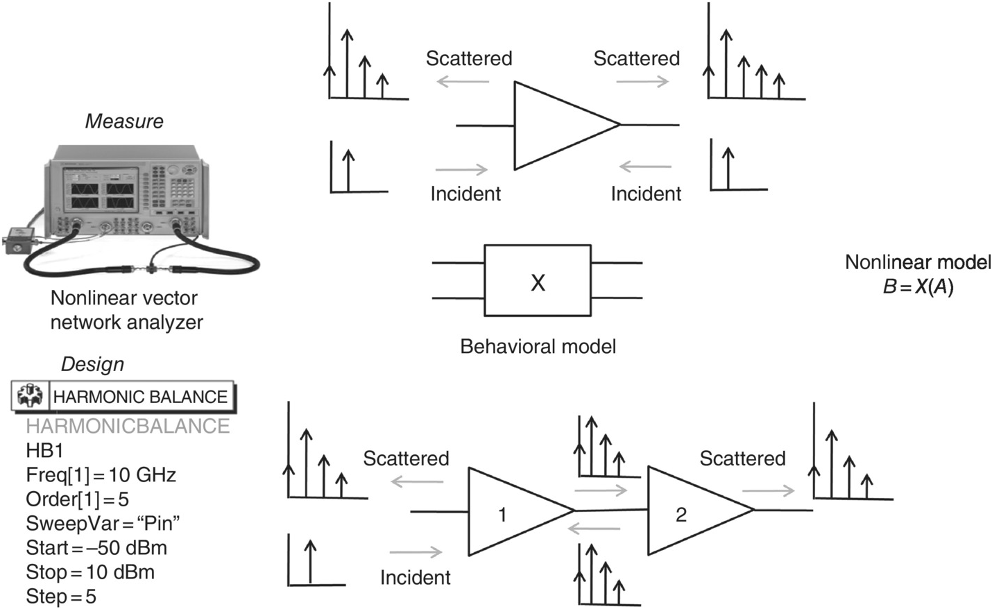
Figure 4.1 Large-signal frequency-domain behavioral modeling paradigm.
Like S-parameters, the models considered here can be identified from measurements, derived from analytical models1, or computed from numerical models in a circuit simulator. The types of required measurements are made on modern RF and microwave instruments called nonlinear vector network analyzers (NVNA) or large-signal network analyzers (LSNA) [1] [2] [3]. Based on good measurements, the resulting large-signal models of components, such as transistors, can be extremely accurate. Simulation-based nonlinear models can be created in the nonlinear simulator in analogy with how an S-parameter analysis produces a linear file-based behavioral model [4].
A major benefit of such high fidelity nonlinear frequency-domain behavioral models is that they can be shared between component vendors and system integrators freely, without the possibility that the component implementation can be reverse engineered. This feature protects vendor intellectual property (IP) and promotes its sharing and reuse. This is quite analogous to the case where S-parameters – measured or computed – are provided by manufacturers to represent the performance of a linear component, instead of a detailed equivalent circuit model that could betray a proprietary implementation or design approach.
The systematic set of approximations to the general theory, based on spectral linearization, is introduced in the chapter in a number of places, to enable practical engineering applications to important classes of problems. These simplifications can result in significant savings of measurement time and file-size, reduce hardware system complexity, and enable faster simulations at a minimal cost in accuracy. Multiple approaches to motivating, deriving, and interpreting the formalism are presented.
Finally, the important topic of dynamic memory is introduced, including its importance, some of its symptoms, and several major causes. A powerful extension beyond the static theory is presented in the guise of dynamic X-parameters. It is shown how this general approach can successfully model many important nonlinear dynamic systems showing a wide range of dynamic-to-the-envelope properties when stimulated with wideband modulated signals.
4.2 Signals and Spectral Maps on a Simple Harmonic Frequency Grid
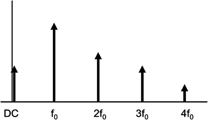
An important application for nonlinear circuit simulation is the analysis of harmonic distortion generated by a nonlinear component, such as a transistor, in response to an excitation at a single fundamental frequency. These response signals, which generally have spectral energy at multiple harmonics of the fundamental frequency, propagate to other components in the circuit and can ultimately get reflected back into any or all of the ports of the device that created them, modifying the outputs in turn. An excitation class that covers most of these cases includes signals incident simultaneously at different ports with frequency components that fall on a grid of discrete non-negative integer harmonic multiples of the fundamental frequency. The DC component is included. A graphical representation is given in Figure 4.2.
We also assume that in response to signals with components at multiple harmonics of the fundamental frequency, the DUT produces scattered waves with nonzero components only on the same harmonic frequency grid. This is usually the case for microwave and RF applications. However, we know from Chapter 1 that it is possible for the DUT to be driven into a chaotic regime where this assumption fails. We also know that parasitic oscillations can be generated and appear in the output spectrum, falling outside the harmonic grid. A phenomenon that is not that uncommon in the PA context is the generation of oscillations at a frequency half that of the fundamental component of the driving frequency excitation, which also does not fall on the grid. We do not consider these cases further here – although the last phenomenon can be handled by minor adaptations of the methods presented here.
In Figure 4.2, the signal magnitudes are indicated by the lengths of the arrows. Each harmonic component of the signal also has a phase that can be well-defined relative to that of the fundamental frequency. This is a consequence of the fact that the frequency components are all commensurate. A set of K frequencies, {fk}, k = 1, …, Kfk,k=1,…,K, are commensurate if there exist nonzero integers, nknk, such that (4.1) is satisfied. For more on commensurate signals see [5].
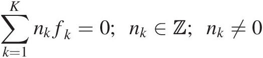 (4.1)
(4.1)4.2.1 Notation for Wave Variables (Phasors) on Harmonic Grid
The complex-valued (for magnitude and phase) incident and scattered wave amplitudes (phasors) now require two indices. The first index refers to the port, and the second to the harmonic index relative to the fundamental. Incident and scattered waves will therefore be labeled according to (4.2):
 (4.2)
(4.2)For example, A2, 3A2,3 is an incident sinusoidal wave at port two at a frequency three times the fundamental, while B1, 2B1,2 is the scattered sinusoidal wave component at port 1 at the second harmonic of the fundamental.
By varying the complex amplitudes of the incident waves’ phasor components at each harmonic of the fundamental frequency and measuring the complex amplitudes of the scattered waves at each port, p, and harmonic frequency index, k, we can build up the set of complex-valued nonlinear algebraic maps of the form (4.3). This set of maps2 defines the behavior of the DUT under all steady-state conditions consistent with our previous assumptions.
To be more complete we need to treat the DC components consistently with the RF components. In the end, it is the actual signals – waveforms – that matter, and the DC components are as important as the RF. Adding the bias stimulus response interactions to those of the RF, we obtain a system of nonlinear functions that define the steady-state behavior of the component. A simple example is given in (4.4). The superscripts in (4.4) simply label the type of value returned by the respective functions (e.g., complex-valued scattered wave, real-valued current, and real-valued voltage, respectively). This notation is standardized in [6].3
 (4.4)
(4.4)In (4.4) there are many independent variables. These include the DC applied voltage at port one, V1; the incident waves at port one at each positive harmonic frequency, A1,1 – A1,N; the DC applied current at port 2, I2; and the incident waves at port two, A2,1 – A2,N.
The scattered RF waves at each port depend nonlinearly on the applied port biases, V1 and I2, and also on each complex-valued phasor of the incident RF signals at each port. Likewise, the DC responses of the DUT, current I1I1 and voltage V2V2, depend on all of the RF incident signal complex amplitudes, as well as applied biases V1 and I2, respectively. Note that this is different from the typical S-parameter situation where the DC conditions are taken to be independent of the applied RF signals since the RF signals are assumed to be arbitrarily small.
The system defined by equations (4.4) is really not much more than book-keeping at this point. For this two-port example there are 2N + 2 nonlinear functions of 2N + 2 variables. The model definition is not complete until all the functions F(B), F1(I), and F2(V) are specified mathematically or otherwise identified from data associated with the component. Even so, the structure of (4.4) makes clear that cross-frequency stimulus-response interactions are taken into account. For example, the third harmonic of the scattered wave at port two depends on the complex value of the second harmonic wave incident at port one. Thus harmonic time-domain load-pull under steady-state large-signal conditions is covered by the system of equations (4.4).
4.3 Time-Invariant Large-Signal Spectral Maps
A fundamental property of components such as transistors, power amplifiers, nonlinear resistors, etc.4 is that of time invariance, discussed in earlier chapters. We saw in Chapter 3 that for linear components the S-parameter mathematical relationship between incident and scattered waves is automatically consistent with the time-invariance principle. This is not true in the nonlinear case, as we will see in section 4.3.1. Since a model inconsistent with the time-invariance property of the physical component must give wrong answers, it behooves us to properly ensure this property is correctly implemented.
Referring to the previous example of (4.4), we will show not all possible functions F(B), F1I , and F2V
 are consistent with the mathematical representation of the time-invariance property. In fact, most are not. The restriction of such functions to those spectral maps obeying the time-invariance property results in X-parameters. This could be taken as the fundamental definition of X-parameters. We will derive these restrictions in Section 4.3.1
Other frequency-domain large-signal behavioral models also obey the time-invariance property. One of these, the Cardiff Model, will be described in section 4.9.2.
4.3.1 Derivation of Time-Invariant Spectral Maps
We don’t need to restrict ourselves to periodic signals for the statement of time invariance, and we drop the port indices for simplicity. We assume the DUT produces an output signal, b(t)bt, when stimulated by an incident signal, a(t)at. A time-invariant DUT means that for an incident signal, a(t − τ)at−τ (the same signal as before but now delayed by an arbitrary time, ττ), the resulting output signal must be b(t − τ)bt−τ (the same response as before but delayed by precisely the same time, ττ).
Returning to our case of periodic stimulus and response, we can write the time-invariance condition in terms of the Fourier coefficients of the incident and scattered periodic signals. We recall that a time-shift, ττ, produces a phase-shift, ejkω0τejkω0τ, for the kth harmonic term of the Fourier series of a periodic signal. This results in the following frequency-domain expression of time invariance for one of the equations of (4.4).
 (4.5)
(4.5)Since (4.5) must hold for all real values of ττ, we choose the particular value given in (4.6). The selection of ττ according to (4.6) can be interpreted as selecting the phase reference to be one of the system’s signals, and that signal is A1, 1A1,1. This has the effect of phase-normalizing each harmonic coefficient of the incident and scattered waves to the phase of A1, 1A1,1, and in particular results in (4.7).
 (4.6)
(4.6)Equation (4.5) can now be recast as (4.8), using the notation P = ejϕ(A1, 1)P=ejϕA1,1.
 (4.8)
(4.8)Equation (4.8) shows that the principle of time invariance restricts the functional form of the spectral mappings to those that change only by a multiplicative phase factor when the arguments to the function are appropriately transformed (phase-shifted) according to their harmonic indices. Exercise 4.1 explores cases where (4.8) is not satisfied. Given (4.7), we can therefore define X-parameter functions as in the bottom of (4.8). Notice that the X-parameter functions, denoted for now by Xp, kXp,k, are defined on a set of independent variables of dimension one fewer than the original mappings Fp,kB . This follows because only the real-valued quantity |A1, 1|A1,1, rather than the general complex quantity A1, 1A1,1, enters the domain of the Xp, kXp,k functions. The final complex coefficient of the scattered wave is obtained by multiplying the value of the X-parameter function by the appropriate phase factor depending on the harmonic index of the scattered wave.
4.3.2 Graphical Representation of Time-Invariant Spectral Maps
The evaluation of an X-parameter model makes explicit use of the time-invariant spectral mapping condition given by (4.8). For example, consider the case of a two-port DUT with signals incident at port one at the fundamental frequency, and simultaneously at port two with components at the fundamental frequency, second, and third harmonics. These four phasors are shown in the top row of Figure 4.3. The length of a vector indicates its magnitude, and the angle represents the phase.

Figure 4.3 Phase normalization of incident waves to the reference stimulus.
Since ϕ(A1, 1)ϕA1,1, the phase of A1, 1A1,1, is not zero, the X-parameter functions that appear in the bottom of (4.8) can’t be evaluated. The prescription of (4.8) requires that we first phase-shift the kth spectral components of the incident waves by k times the phase of A1, 1A1,1 in the clockwise direction. This is accomplished by multiplying each variable Ap, kAp,k by P−k = e−jkϕ(A1, 1)P−k=e−jkϕA1,1. The second harmonic terms will therefore be phase-shifted twice as much as the fundamental component, and third harmonic terms three times as much, etc. DC terms (not shown in the figure) are not modified – consistent with DC being the “zeroth” harmonic, or k = 0. The resulting phasors, denoted by Ap,kn=Ap,kP−k , define the reference stimulus.5 These are shown in the bottom of Figure 4.3, emphasizing the relative phase rotations of the various harmonic components. In the time domain, the reference stimulus is simply the original set of periodic incident waveforms translated in time with respect to the original waveforms by a time, ττ, given by (4.6) [7].
The X-parameter functions of (4.8) can be evaluated at the reference stimulus because A1, 1(n)A1,1n is a real number. We denote by reference response the values of the scattered waves returned by the X-parameter functions evaluated at the reference stimulus. The corresponding phasors of the reference response are denoted Bp,kn . Since the DUT is nonlinear, there will generally be scattered waves at each port with nonvanishing components at multiple harmonics beyond those of the incident signals. Values for four of these scattered phasors of the reference response are shown in the top part of Figure 4.4.

Figure 4.4 Phase denormalization from the reference response to the actual response.
Finally, the desired Bp, kBp,k values (corresponding to the actual Ap, kAp,k incident waves) are obtained by a phase denormalization process applied to the reference response. This is accomplished by a phase-rotation in the counterclockwise sense (complex multiply by Pk = ejkϕ(A1, 1)Pk=ejkϕA1,1) of the values returned by the X-parameter functions according to (4.8). In the time-domain, this corresponds to the appropriate delay of the periodic reference response by the precise amount, ττ, by which the incident signals were delayed compared to the reference stimulus.
In summary, we have taken an arbitrary periodic stimulus, time-translated it to a reference condition where the phase of A1, 1A1,1 can be taken to be zero, evaluated the X-parameter functions, and time-translated the result back to obtain the final periodic response. Since this is a manifestly time-invariant process, we are guaranteed the DUT’s time-invariant behavior is built in to the mathematical description through the X-parameter formalism.
4.4 Large-Signal Behavioral Modeling Framework in Wave-Space
The steady-state nonlinear behavior of RF and microwave components are defined in terms of time-invariant spectral maps defined in wave-space – with DC conditions specified in terms of real-valued currents and voltages that also depend on the RF incident waves. Schematically, this is represented by Figure 4.5, for an example of a component that we label, simply, as a (frequency) converter.

The example of Figure 4.5 has three RF ports, labeled 1 through 3, as well as a DC port, labeled 4. The incident RF waves are indicated by Ap, where the port index p ranges from 1 to 3. The waves have multiple harmonic components, but these second indices are suppressed in the figure for simplicity. The incident waves and the DC applied voltage, V4, are taken as the independent variables. The scattered waves, Bp, and the DC current, I4, are given by X-parameter relations such as (4.8). For example, the RF outputs at port 2 are specified by the X-parameter expression (4.9), for Ap,kn=Ap,kP−k
 (4.9)
(4.9)For port 4, the expression for the bias current response is given in (4.10). In the general case, there are both DC and RF input and outputs at each port.
 (4.10)
To model a particular device, the abstract constitutive relations (4.9) and (4.10) – as well as those for every X-parameter function corresponding to Figure 4.5 – must be identified from measured (or simulated) input–output characteristics of the component. In principle, this can be obtained by an exhaustive process of applying DC and RF sources at each port and varying the magnitudes and phases of all RF components and the value of the applied bias voltage, V4, and acquiring the resulting responses. The outputs can be fitted with smooth functions of all the inputs or tabulated and interpolated by the simulator during simulation. This process is limited by “the curse of dimensionality,” however. That is, it becomes exponentially complex in the number of independent variables. To deal with this, we present systematic approximations that can be used to more conveniently apply the X-parameter principles to many important cases of practical interest, starting in Section 4.6.
4.5 Cascading Nonlinear Behavioral Model Blocks
How is it possible to combine, in analogy with linear S-parameters, multiple large-signal behavioral functional blocks to simulate a more complicated nonlinear circuit or system? We illustrate the concept by connecting port 2 of the converter block of Figure 4.5 to the input of a simple power amplifier (PA) block in Figure 4.6. The input port of the PA is labeled port 5, and the PA output is labeled port 6. The scattered waves at port 5 of the PA are defined by X-parameter constitutive relations that depend only on the incident waves (and biases, not shown) at ports 5 and 6.

Figure 4.6 Cascading large-signal functional blocks in wave-space.
To solve the circuit of Figure 4.6, Kirchhoff’s Current Law (KCL) and Kirchhoff’s Voltage Law (KVL), must be applied at the node connecting the two blocks. These conditions impose constraints on the sets of incident and scattered waves, given by the simple relationships (4.11). Specifically, at the solution of the circuit, the incident waves at port 2 must be equal to the scattered waves from port 5, and the scattered waves from port 2 must be equal to the incident waves at port 5. These equalities must hold separately for each harmonic index, k, k = 1,…,N. That is, (4.11) is a set of 2N equations, or if including DC terms, 2(N + 1) equations. It is a simple matter to prove that (4.11) is equivalent to the circuit laws, KVL and KCL, when expressed in terms of wave variables using equations 3.1:
 (4.11)
The solution for the entire circuit is given by eliminating the scattered wave variables and solving the set of self-consistent implicit nonlinear equations for the incident waves A2, k and A5, kA2,kandA5,k for k = 1,…,N, given by (4.12). Contrary to the case of cascaded S-parameters considered in Chapter 3, because the present problem is nonlinear, no closed form solution can be found in general for the X-parameters of the cascade as a function of the X-parameters of each block. The solution to (4.12) is therefore obtained numerically by the nonlinear circuit simulator:
 (4.12)
Of course most available circuit simulators first convert the wave variables in (4.12) to currents and voltages, using equations (3.2), and then solve the resulting implicit nonlinear equations in current-voltage space.
In fact, the simple relations (3.1) and (3.2) between wave variables and current-voltage variables enable functional blocks to be cascaded with nonlinear (and linear) functional blocks expressed in wave-space and/or conventional current-voltage space. That is, large-signal frequency-domain behavioral model functional blocks are completely compatible with distributed passive elements, lumped nonlinear elements defined in the time domain, and “compact” nonlinear transistor models. However, the present formulations of X-parameters and similar frequency-domain nonlinear behavioral models (e.g., the Cardiff Model – see Section 4.9.2) are presently limited to harmonic balance and circuit envelope analyses or their subsets (S-parameters, small-signal mixer analysis, etc.).
It should be stressed that the cascadability of these functional blocks depends only on the accuracy of the sampled constitutive relations of each block. The results for the cascade follow directly by applying only the circuit laws. No additional approximations are required. The cascadability becomes arbitrarily accurate by taking into account enough harmonic components of the incident and scattered waves at sufficiently many complex values of the independent incident wave variables.
4.6 Spectral Linearization
4.6.1 Simplification for Small Mismatch
The considerations used for the definition and application of X-parameters and related approaches described thus far apply to the steady-state behavior of time-invariant nonlinear components with incident and scattered waves on a harmonic frequency grid. The generality of the formalism comes at the cost of considerable complexity. Each spectral map is a nonlinear function of every applied DC bias condition and all the magnitudes and phases of each spectral component of every signal at every port of the component. Sampling such behavior in all variables for many ports and harmonics would be prohibitive in terms of data acquisition time, data file size, and model simulation time.
Fortunately, in most cases of practical interest, only a few large-signal components need to be considered with complete generality, while most spectral components can be considered small and can be dealt with effectively by methods of perturbation theory. In fact, as stated previously, S-parameters are the limiting case where all RF signals are considered small. Specifically, we can apply the following methodology, depicted in Figure 4.7.
– Identify the few large tones that drive the nonlinear behavior of the system.
– Identify the nonlinear spectral maps defined when only these few large tones are incident on the DUT. This nonlinear spectral map represents the specific steady-state of the system, designated the large-signal operating point (LSOP).
– Linearize the spectral maps around this LSOP defined by the few important large tones.
– Treat the remaining small signals as small perturbations, using superposition appropriately, based on the above linearized maps around the LSOP.
This methodology approximates the complicated general multivariate nonlinear maps, BkBk, with much simpler nonlinear maps, XkF , defined on the few preselected large tones only, and simple linear maps, Xk,k’SandXk,k’T
 , which account for the contributions of the many small amplitude tones. These approximations result in a dramatic reduction of complexity while providing an excellent description for many important practical applications. The details of the equations appearing in Figure 4.7 will be derived and discussed further in Section 4.6.2.

Figure 4.7 Illustration of spectral linearization approximation. The equations will be discussed in more detail in Section 4.6.2
The simplest such approximation is to assume there are no large RF signals that need to be treated fully nonlinearly. The LSOP is therefore just the DC operating point. All the RF components can then be treated with perturbation theory, by linearizing around the DC operating point. This is just the S-parameter approximation of the previous chapter.
4.6.2 Simplest Nontrivial X-Parameter Case
Beyond S-parameters, the next simplest case of X-parameters involves one large RF signal that is treated generally while the remaining spectral components are treated as small. This is often the case for power amplifiers, at least those “nearly matched” to 50 Ω, where the main stimulus signal is a narrow-band modulation around a fixed carrier incident at the input port. The DUT response generally includes several harmonics. If the DUT is not perfectly matched at the output port, there will be small reflections at the fundamental and the harmonic frequencies back into the output port of the DUT. These small reflected signals will be treated as perturbations to simplify the description. Similarly, scattered waves at the harmonic frequencies at the input could be reflected back into the DUT if it is not perfectly matched at the source. These incident signals can also be treated as small in many applications. The validity of the approximation depends on whether these signals are small enough so that their contributions do not affect the LSOP. This is quite analogous to the condition on an RF signal to be small enough such that it does not change the DC operating point of a device for a valid S-parameter measurement, as discussed in Chapter 3. In Section 4.9 we will consider multiple large signals, in particular to deal with arbitrary load-dependence for large mismatch at the output port (load-pull) and two large incommensurate tones for mixer analysis.
4.6.2.1 Digression: Double-Sided Spectra and Spectral Linearization
So far we have simply assumed our phasor description corresponds to single-sided spectra. That is, the complex value, Ap, k or Bp, kAp,korBp,k, is associated with ejkω0tejkω0t for positive values of the harmonic index k, for ω0ω0 is a positive angular frequency. The spectral maps take complex amplitudes for positive frequencies into scattered wave amplitudes at positive frequencies (and DC). The simultaneous presence of signals incident at multiple frequencies on a nonlinear device, however, creates self-mixing, with signals scattered at frequencies corresponding to the sum and difference frequencies of the incident signals. For example, if we have signals simultaneously incident at positive frequencies f1 and f2f1andf2, we will get scattered signal components at frequencies f1 ± f2f1±f2. This is fine for f1>f2f1>f2, and we can map incident phasors associated with positive frequencies into scattered phasors also associated with positive frequencies. But we must consider also the case where f1 < f2f1<f2. If we restrict ourselves, as we have so far, to positive frequencies – single-sided spectra – we will have to be careful about how we consistently deal with some of the resulting mixing terms.
For this and other reasons, it is convenient to expand the domain of incident and scattered complex amplitudes to double-sided spectra. That is, we consider signals with positive and negative frequencies incident and scattered by the DUT.
We now have the situation depicted in Figure 4.8.

Figure 4.8 Double-sided spectra on a harmonic grid.
Formally, this means we have to consider the arguments to all spectral maps to include negative frequency components as well as positive. Thus we must generalize equations (4.3) to a form given by (4.13). Similar conditions apply to (4.4). We note (4.13) also depends on the DC bias but this is suppressed for simplicity.
Not only do the arguments of (4.13) include phasors corresponding to negative frequencies on a double-sided harmonic grid, but the index k for the scattered wave harmonic is now permitted to take negative integer values as well as positive integer values. While this appears to increase the complexity, we will be able to use this approach as a simple starting point from which to derive the formalism of spectrally linearized X-parameters for small mismatch.
We now define spectral linearization of double-sided spectral maps. We assume all spectral components except A1, 1 and A1, − 1A1,1andA1,−1 are small so we can expand (4.13) in a complex Taylor series. We write, noting the summations omit terms with joint values of (q = 1, l = ± 1)q=1l=±1:
 (4.14)
Here we have introduced the notation large-signal operating point stimulus, or LSOPS, to refer to the set of large-signal incident waves (and DC applied biases) in the absence of the small signals. Note the summation in (4.14) excludes the phasors A1, ± 1A1,±1 that are arguments of the LSOPS. The reference large-signal operating point stimulus, RefLSOPS, is obtained from the LSOPS by phase-normalizing the arguments. This transformation brings out the phase factors Pk and Pk − k‘PkandPk−k’ in the respective terms using the time-invariance principle discussed in Section 4.3. The derivation of the last equality of (4.14) is left as an exercise.
We have introduced the notation Xp,kF to denote the X-parameter function evaluated at the RefLSOPS. The symbols X(d)Xd denote the partial derivatives of the double-sided spectral maps evaluated at the RefLSOPS.
Now we can get back to real signals by imposing conjugate symmetry. That is,
 (4.15)
We now return to the single-sided spectral representation. We restrict ourselves to positive indices but invoke (4.15) to define the contributions from negative frequencies. We can therefore re-express (4.14) as (4.16) where X(S)XS and X(T)XTare defined for positive indices as the corresponding terms of X(d)Xd for only positive indices. For notational simplicity, in this and what follows, we omit the double summation sign even though we are summing over two indices, q and l. In (4.16) the summation does not include the term for which both q = 1 and l = 1 together.
 (4.16)
Equation (4.16) is the classical form of the spectrally linearized maps around a single large tone at the fundamental frequency at the input port of a nonlinear DUT [6]. This is defined in terms of single-sided spectra for positive frequencies only, since this is what is measured. Unlike S-parameters, there are independent contributions linear in A and also linear in A*, with separate coefficients X(S)XS and X(T)XT, respectively. The terms X(F)XF, X(S)XS, and X(T)XT are nonlinear functions of their arguments, namely the applied DC biases and (phase-normalized) complex amplitudes of the RF signals. We can now properly identify the terms of (4.16) with the corresponding labels in Figure 4.7.
Expressions similar in form to (4.16) hold when the RefLSOPS is more complicated than the case considered in this section, as we will see when considering two large tones for “load-dependent” X-parameters and for mixers in Section 4.9.
4.6.3 Identification of X-Parameter Terms from Measured Data
4.6.3.1 Ideal Experiment Design and Identification by Offset Phase Method
The objective is to identify (extract), for each specific RefLSOPS of the DUT, all of the X-parameter values, specifically Xp,kF,Xp,k;q,lS,andXp,k;q,lT , that enter equation (4.16). We will treat this algebraically in this section and provide a geometrical interpretation in Section 4.6.7.
It is assumed for now (this restriction will be removed in Section 4.6.3.2) that the source and the measurement instrument are ideal. Specifically, we assume an ideal incident tone at port one and that no signals generated by the DUT in response to the large excitation signal are reflected back into the DUT.
For each port number, p, and harmonic index k, the ideal experiment design for each RefLSOPS consists of a sequence of three distinct RF excitations, labeled by integer m and measurements of the corresponding scattered wave, Bp,km for each excitation.
The first excitation is a single large tone of complex amplitude A1, 1A1,1, applied at port one, with measurement result denoted by Bp,k1 . The second excitation involves application of the same large-amplitude tone, A1, 1A1,1, and, simultaneously, the application at port q and harmonic index l of a small perturbation tone with complex amplitude Aq,l1
 . The measurement result for this case is Bp,k2
 . Finally, the third excitation is of the same type as the second experiment, but with a distinct phase for the small tone at port q and harmonic index l, which we label as Aq,l2
 . The measurement result is Bp,k3
 .
.
Using (4.16), we obtain three linear equations for the unknown X-parameter values Xp,kF,Xp,k;q,lS,andXp,k;q,lT , in terms of known excitations A1,1,Aq,l1,andAq,l2
 and the measured values Bp,k1,Bp,k2,andBp,k3
 shown in equation (4.17).
 (4.17)
This procedure is then applied, separately, for small perturbation tones at other ports and harmonic indices (different values for the indices q and l), and the entire process repeated for each distinct RefLSOPS for which the X-parameter values are desired. The phases of the small tones, Aq, lAq,l, in (4.17) can be arbitrary,6 but the system of equations is better conditioned when the phase difference between Aq,l1andAq,l2 is close to 90 degrees. More than two phases for the applied small tones, Aq,lm
 , can be used as stimuli and the resulting augmented system (4.17) solved for the X-parameter values in a least squares sense in order to reduce the effect of measurement noise.
4.6.3.2 X-Parameter Identification in an Imperfect Environment
The method of Section 4.6.3.1 describes X-parameter identification in a perfect world. However, an actual microwave source, when used at high power conditions, may generate its own complex-valued harmonic distortion components, so the intended ideal excitations of the previous section may not be realized precisely. The output of the DUT in response to such a “dirty source” is therefore a combination of its response to a pure tone and that of the amplified spurious signals that contaminated the input. In addition, the measurement HW may not present a perfect 50 Ω environment to all signals generated by the DUT in response to the large-signal excitation. Both of these nonidealities, if not properly accounted for, create errors in the values of the X-parameters that we wish to attribute to the DUT.
An extension of the method described in Section 4.6.3.1 was developed in [8] for measuring and identifying X-parameters using nonideal HW. The method can be used to characterize the imperfect source and then “predistort” it so that it produces a pure, single-tone input, or, equivalently, correct the DUT response to a dirty source and imperfect match, in order to predict the DUT response to an ideal source or sources. The method is a practical way to calibrate out the imperfections of the source and measurement HW so as to properly return X-parameters that can be regarded as intrinsic properties of the DUT on its own, rather than the combined source-DUT-instrument system. A schematic representation of the idea is given in Figure 4.9.

Figure 4.9 Method to identify X-parameters in an imperfect environment
Despite the imperfect environment, the complete set of X(S) and X(T) parameters can be identified from a global analysis of the measured data from the entire set of experiments of the type described in Section 4.6.3.1 for all values of small tone indices q and l. The desired stimulus (a large pure tone at the input) is subtracted from the actual measured stimulus that consists of one large tone and several complex harmonic components. This results in an “imperfection” signal with small components at each harmonic of the fundamental. This imperfection signal is then used with the previously identified X(S) and X(T) parameters to calculate corrections to the measured response so as to return the actual DUT response to the ideal large stimulus.
This method is particularly effective in X-parameter applications where (far from 50 Ω) loads are controlled and presented to the DUT by the HW system (e.g. with a tuner or an active source at the output port), but where harmonic loads may be uncontrolled and vary as the fundamental load is changed. This will be described in the context of an example in section 4.9.1.5. The method, so applied, is used to calibrate out the harmonic terminations to help present X-parameters referenced to ideal excitations under known loads with perfectly matched harmonic terminations.
4.6.4 Example: X-Parameters of a Two-Port Amplifier with Small Mismatch
A simple and illustrative example of the basic X-parameter formulation (4.16) is a nearly matched two-port power amplifier driven by a large signal at port 1. Neglecting any harmonics, for simplicity, (4.16) reduces to (4.18).
 (4.18)
Thus a two-port, in this simple “fundamental only” approximation, has six X-parameter functions, whereas a linear two-port is described by only four S-parameters. The six X-parameter functions in (4.18), and therefore the scattered waves, Bp, 1Bp,1, depend on |A1, 1|A1,1 (shown) and also depend on the DC bias conditions, but we suppress the DC arguments for simplicity.
In Figure 4.10, we plot the values of the three X-parameter functions, X2,1F,X2,1;2,1S,andX2,1;2,1T in (4.18), that contribute to B2, 1B2,1, versus the input port drive, |A1, 1|A1,1. The function X2,1F
 is divided by the magnitude of the incident wave to make the result unitless, like the other two functions shown.

Figure 4.10 Some X-parameter functions of a power amplifier.
We observe two things about the various X-parameter functions. As the power of the incident signal diminishes, so does the value of the X(T)XT term. In fact, in the limiting case of vanishing power, the X(T)XT term goes all the way to zero, as we’ll see in Section 4.8. This should be no surprise. After all, we know that in the small-signal limit, the S-parameter formalism of Chapter 3 is a complete description. Since the X(T)XT terms in (4.18) contribute to the scattered waves terms proportional to the conjugates of the incident phasors, and these conjugate terms don’t appear in the S-parameter description, we logically conclude all X(T)XT terms must vanish in the small-signal limit.
On the other hand, at large incident power levels at port 1, the magnitudes of the X(T)XT terms can increase to the point where they can become comparable to, or even exceed, the magnitudes of the X(S)XS terms. The X(T)XT terms are therefore just as important as the X(S)XS terms at very high incident drive levels. This is true no matter how small the incident signals are at port two when the DUT is driven hard at port one.
4.6.4.1 X(S) and X(T) Functions in Terms of Double-Sided Sensitivities
If we want, we can relate X(S)XS and X(T)XT defined on positive frequencies, to the double-sided derivatives of the double-sided spectral maps as follows [9]:
Comparing (4.16) with (4.14) we have, for k, l >0:
 (4.19)
In (4.19) we again use the superscript “(n)” to denote phase-normalized waves. Using (4.15), we also find
 (4.20)
The double-sided expression (4.14) is an analytic function (in the sense of complex variable theory) of each complex phasor Aq, lAq,l. For single-sided expressions, however, the spectral map (4.16) is nonanalytic. That is, we must differentiate with respect to Ap, kAp,k and Ap, k∗Ap,k∗ independently in this expression. The coefficients, X(S)XS and X(T)XT, correspond to partial derivatives of the single-sided spectral map with respect to Aq, lAq,l and Aq, l∗Aq,l∗, respectively.
4.6.5 Origins of the Conjugate Terms
The appearance in (4.16) of terms linear in both AA and A∗A∗ is perhaps surprising. The preceding analysis shows that the origin of the A∗A∗ terms is the mixing of the small amplitude negative frequency components back into the positive domain. Of course there is no mixing when the DUT is perfectly linear, so these terms have no analogue in the simple S-parameter world. Simply making S-parameter measurements at high input power levels (e.g. so-called “hot S22”) cannot account for such terms and their measurable consequences [10].
Expression (4.16) allows us a more detailed interpretation of Figure 4.7. We suppress the port indices on the diagram for simplicity. The top line of Figure 4.7 shows a single-sided spectral map from four RF signal components (plus DC) into an output spectrum. The nonlinear function depends on the complex values of all independent variables. The approximation made now is to designate one of the incident RF signals as large and the remaining ones as small. Of the four incident signal components (apart from DC), the one at the fundamental frequency is supposed large and the others small. This is indicated by the groupings in the top left of Figure 4.7.
The approximate decomposition of the scattered waves, BkBk, using (4.16), is indicated in Figure 4.7. The simple nonlinear map, designated by XkF , depends only on the DC and the single real number corresponding to the magnitude of the large tone. This is much simpler than the full nonlinear map that depends on all variables. The phase factor PkPk multiplies the X-parameter function to ensure the map is properly time invariant. Note how close the output spectrum on the right column second row is to the full result (top row). The minor differences are now nearly completely accounted for by the contributions from the multiple linear maps, Xk;lSandXk;lT
 . Each small tone, AlAl, contributes linearly to the response around all harmonics due to contributions weighted by X(S)XS terms and also linearly in Al∗
 with contributions weighted by independent X(T)XT terms. Equivalently, there is a contribution at each harmonic, k, linear in each of the AlAl and each of the Al∗
 terms. The “wiggly” nature of the lines indicates the phase-dependent contributions of the complex numbers, added as vectors. The length of the sum of all the vectors at each frequency depends on each of their phases and magnitudes; they add vectorially.
4.6.5.1 More on the Origin of Conjugate Terms: An Example with a Cubic Nonlinearity7
A concrete example is now provided as another illustration of the origins of the conjugate terms. We consider the simple case of a static algebraic nonlinearity (e.g., a polynomial) in the time domain and compute the mapping in the spectral domain. We start by considering a system described by a simple instantaneous nonlinearity containing both a linear and cubic term. We look at the following three cases, for which the analysis can be computed exactly. The first case is the linear response of this nonlinear system around a static (DC) operating point. This is the familiar condition for which linear S-parameters apply. The second case is the linearization of the system around a time-varying large-signal operating state, with the time variation and perturbation having the same fundamental period. The third case is a simple generalization of the second where the perturbation is applied at a distinct frequency compared to the fundamental frequency of the periodically driven nonlinear system.
The objective is to look at the linearized response of the system in the (single-sided) frequency domain and demonstrate that the relationship between the perturbation phasor and the response phasor is not an analytic function in cases 2 and 3, namely when the nonlinear system is driven. That is, these examples illustrate the simultaneous presence of the perturbation phasors and their complex conjugate phasors, with distinct coefficients, in the response of a nonlinear driven system to additional injected signals.
The nonlinearity is described by (4.21). The signal, x(t)xt, is written in (4.22) as the sum of a main signal and a perturbation term, assumed to be small. We will calculate, to first order in the perturbation, the response of the system (4.21) to the excitation (4.22). We will consider three cases.
Case 1
 (4.23)
In this case, shown in (4.23), the main signal, x0(t)x0t, is just a constant value (a DC term) while the perturbation is a small tone at angular frequency ωω. The constant A is real and δδ is a complex number of small magnitude that allows for the phase of the perturbation to be arbitrary. The total signal is obviously real.
The first order response is computed in (4.24). The approximation becomes exact as Δx(t)→0Δxt→0
For this case, the conductance nonlinearity, f′(x0)f′x0, is evaluated at the fixed value x0 = Ax0=A, where, using (4.21), we obtain (4.25), where G(A) is defined as being,
Substituting (4.25) into (4.24) and using (4.23) we obtain (4.26):
 (4.26)
If we look at the complex coefficient of the term proportional to ejωtejωt we find it is given simply in (4.27):
 (4.27)
Since (4.26) is a linear input–output relationship with constant coefficients, the complex Fourier component at the output frequency is linearly proportional to the complex Fourier coefficient of the input small-signal phasor. In fact we can read off the frequency-domain phasor relationship (4.28), or equivalently (4.29), where the gain, G(A)GA, is given by (4.25) and X(ω)Xω is the complex input phasor corresponding to the positive frequency component of the small perturbation tone. We note in this case the gain, G(A)GA, depends nonlinearly on the DC operating point, through (4.25), but is constant in time.
 (4.29)
Case 2
 (4.30)
This time we take x0(t)x0t to be a pure sinusoid given in (4.30). There is no loss of generality by taking AA to be real, which is equivalent to taking the phase of the main signal at time zero to be zero. We can interpret δδ as the relative phase between the main signal and perturbation signal at the same frequency.
We go through the same procedure as in Case 1 to derive the conductance, but this time it is evaluated at the periodically time-varying operating condition (essentially the LSOPS) according to (4.31). The second form follows from the simple trigonometric identity cos2ωt=12+cos2ωt2 .
.
 (4.31)
Using (4.31) to evaluate (4.24) for this case, we obtain (4.32):
 (4.32)
This time we get contributions proportional to ejωtejωt and e3jωte3jωt, and their complex conjugates, four terms in all. If we restrict our attention, as in case 1, to output terms proportional to ejωtejωt, we obtain the coefficient given in (4.33):8
 (4.33)
We observe that the output phasor at frequency ωω is not proportional to the input phasor, δδ, at frequency ωω but instead has distinct contributions proportional to both δδ and δ∗δ∗. That is, the linearization of the nonlinear system around the periodically time-varying operating point determined by the large tone, is not analytic in the sense of complex variable theory. If it were analytic, (4.33) would depend only on the complex variable, δδ, and not on both δδ and δ∗δ∗.
Taking the ratio of the complex output Fourier Coefficient to the input Fourier coefficient, we obtain the result (4.34), where ϕ(δ)ϕδ is the relative phase of the main and perturbation signal:
 (4.34)
Therefore, unlike linear S-parameters (and therefore unlike the case (4.29)), this small-signal ratio is not independent of the phase of the small perturbation tone. That is, the large tone creates a phase reference such that the response of the system to even a very small perturbation around the large-signal time-varying state depends explicitly on the relative phase of the perturbation tone and the large tone.
This should come as no surprise, if we think of the large tone as turning on and off, smoothly and periodically, an active device. Even the small-signal scattering of a second tone will clearly depend on where in the time-varying cycle (phase) the device happens to be when the scattering occurs.
Case 3
 (4.35)
Here we allow the frequency, ω1ω1, of the perturbation tone to be distinct from the frequency, ωω, of the main drive signal. We go through the analysis once again. The time-varying conductance is the same as before, with the only difference being the frequency of the small perturbation term in parentheses in the rightmost factor of (4.36):
 (4.36)
Since ωω and ω1ω1 are distinct, there are more frequency components generated then in the previous cases. We may write ω1 = ω + εω1=ω+ε and look at the terms proportional to ej(ω + ε)tejω+εt and ej(ω − ε)tejω−εt. We obtain, respectively, (4.37) and (4.38):
 (4.37)
 (4.38)
Terms (4.37) and (4.38) represent the single-sided spectrum of the lower and upper sidebands of the intermodulation spectrum of the system (4.21) for excitation (4.22) defined by (4.35) around the fundamental frequency of the main signal.
We note that as the tone spacing, εε, goes to zero, both these contributions overlap (add) at the frequency ωω of the drive signal, and we recover the results of case 2 (equation (4.33)).
The ability to separate the terms proportional to δδ from those proportional to δ∗δ∗ obtained by this “frequency offset” method remains true for the more general dynamic nonlinear system beyond our simple example. In the general case, the upper and lower sideband phasors depend explicitly on the frequency offset, εε (unlike the simple example here). Case 2 can be recovered using case 3 for each sideband for finite εε and then taking the limit ε→0ε→0. This indicates that it is possible to extract each upper and lower sideband term (per harmonic frequency component) from measurements of the system response to a small tone with a single, arbitrary phase rather than introduce two (or more) distinct phases to extract the two terms when they appear at the same frequency as in (4.17). We will formalize this concept in Section 4.6.6. On the other hand, there are now measurements to be made at distinct frequencies for the upper and lower sidebands, so this method does not lead to fewer measurements than that of case 2.
Examination of case 3 reveals that the complex conjugate term results from intermodulation or mixing, a consequence of nonlinearity, and disappears as the size of the drive signal decreases to zero. This is evident by evaluating (4.37) and (4.38) (or even (4.33) for case 2) as the drive A→0. The terms proportional to δ* vanish and the terms proportional to δ reduce to the result we would get for a linear system with constant gain α.
In the limit ω→0ω→0, case 3 reduces to case 1, equation (4.27), corresponding to the system linearized around a static operating point. This is most easily seen by taking the limit ω→0ω→0 in (4.36). Thus, although the X-parameter model as discussed so far is representative of case 2 (perturbation signals at exact integer multiples of the fundamental drive signal), the origins of the different terms are made more obvious by examining the slightly more general case 3.
4.6.6 Spectrally LInearized X-Parameters in Terms of Sidebands – Offset Frequency Linear Responses
To provide a useful interpretation of the X(S)XS and X(T)XT terms, we consider the slightly more general example of a single large tone at frequency f0 and a second small tone at f1 = 2f0 + εf1=2f0+ε incident simultaneously on the nonlinear DUT [12]. Here εε is a small positive frequency offset. This is illustrated in Figure 4.11.

Figure 4.11 Large tone plus a small tone offset slightly from the second harmonic.
This second tone, injected at port q for definiteness, has small amplitude ΔAq, k‘+ΔAq,k’+, at a frequency εε above the kth harmonic of the fundamental frequency, in the presence of the large tones. The “+” superscript indicates the frequency is slightly more positive than the harmonic. From standard mixer theory, we know there will be small sidebands, both upper and lower, appearing at each port around each of the harmonics of the original spectrum. The complex-valued spectral components are labeled ΔBp,k+ and ΔBp,k−
 for the upper and lower sidebands, respectively, at port p and harmonic index k. This is shown in Figure 4.12.

Figure 4.12 Sidebands created by mixing of time-varying nonlinear DUT with small tone stimulus offset from the second harmonic.
We observe that the response in the vicinity of any harmonic of the fundamental contains three separate contributions. We focus on the responses around the third harmonic for definiteness. The phase of A1, 1A1,1 is suppressed in the figure and the following discussion. The first of the three terms is that of the direct 3rd harmonic response of the DUT to the large tone in the absence of the perturbation. This is just the value of the single-tone response, Xp,3F . The second contribution, just above the 3rd harmonic, is attributable to a second order mixing term, first order in the fundamental frequency of the large tone and first order in the positive frequency component of the perturbation tone. This is the value of Xp,3;q,2S
 times the value of ΔAq, 2ΔAq,2. The third contribution is a sixth order mixing term, fifth order in the DUT nonlinearity, and first order in the negative frequency component of the perturbation. This is the value of Xp,3;q,2T
 times the value of ΔAq,2∗
 (neglecting the phase of A1, 1A1,1).
The mixing order can be inferred from the diagram as follows. The length of the solid horizontal arrows indicate the harmonic order of the fundamental frequency needed to be combined with either the positive or negative first power of the perturbation tone. The length of the right-pointing (positive frequency) and left-pointing (negative frequency) dashed horizontal arrows indicates the frequency multiple of the harmonic at which the perturbation tone is being applied.
There are only two combinations of solid and dashed horizontal lines such that, when added as vectors, fall within an εε neighborhood of the kth harmonic frequency. These terms are identified as the appropriate Xp,k;q,lS and Xp,k;q,lT
 parameters, the proportionality coefficients of the response at port p at the kth harmonic to the perturbation at port q at the lth harmonic in the presence of the large-signal(s) driving the nonlinear component.
As the frequency offset vanishes, these three terms in the vicinity of each harmonic coincide at the same frequency – or collide – and therefore must be added vectorially. Since the perturbations are small, we can consider their combined effects by a superposition of their effect at each frequency individually. The final result is just (4.16).
4.6.6.1 Interpretation of Sensitivity Terms as Sideband Stimulus Response Ratios
The above discussion provides an alternative definition of the Xp,k;q,lS and Xp,k;q,lT
 terms. In words, Xp,k;q,lS
 and Xp,k;q,lT
 are the limiting ratios of the upper and lower sideband responses, respectively, at angular frequency kω0kω0, to a small perturbation tone injected at angular frequency lω0 + εlω0+ε, as ε→0+ε→0+. This is formalized in (4.39). It should again be emphasized that the values of Xp,k;q,lS
 and Xp,k;q,lT
 depend on the RefLSOPS, and therefore on the incident DC bias conditions and value of the large RF signal.
 (4.39)
We note from (4.39) that unlike some Xp,k;q,lS terms (those for which k = l), all Xp,k;q,lT
 terms are related to responses at frequencies distinct from the perturbation stimulus frequency. That means mixing must be occurring for there to be non-vanishing Xp,k;q,lT
 terms. Mixing can’t happen in a linear device. In fact, we show in Section 4.8 that the value of the X(T)XT functions must go to zero when the amplitude of the driving signal goes to zero, or equivalently when the component is linear. This is another explanation for the fact that there are no S-parameter analogues to the X-parameter terms depending on the conjugate phasors of the incident signal components.
4.6.7 Geometrical Interpretation of X(S) and X(T) Terms
In the X-parameter case, for a nonlinear DUT, we have to deal with independent terms linear in both Ap, kAp,k and Ap,k∗ . We consider the case for p = 2 and k = 1 only for simplicity.
We define ΔB2.1ΔB2,1 in (4.40) and (4.41) (compare equations 3.9 and 3.10 for the linear case) where we use the ΔΔ symbol to emphasize these signals are small (whereas the drive signal, A1, 1A1,1 is large).
 (4.40)
 (4.41)
We rewrite (4.41) as
 (4.42)
where θΔA2,1=ϕXS−ϕXT2+ϕΔA2,1−ϕA1,1 .
.
Defining X=ΔA2,1X2,1;2,1S+X2,1;2,1TCosθΔA2,1 and Y=ΔA2,1X2,1;2,1S−X2,1;2,1TSinθΔA2,1
 we have9
 (4.43)
Which is just the standard expression for an ellipse with semi-major axis ΔA2,1X2,1;2,1S+X2,1;2,1T and semi-minor axis ΔA2,1X2,1;2,1S−X2,1;2,1T
 . The phase factor multiplying the last line of (4.42) just rotates the ellipse around its center by an angle related to the phases of A1,1 and the phases of the X(S) and X(T) terms. An example is shown in Figure 4.13.

The extraction from measurements of the X-parameter functions, using (4.17) and the discussion of 4.6.3, can therefore be interpreted geometrically as the identification of a set of ellipses like that given in Figure 4.13 for the particular case p = 2 and k = 1. For each port index p and harmonic index, k, there correspond ellipses with center displaced from the origin by the complex vector Xp,kFPk , with orientation and eccentricity determined by the values of Xp,k;q,lSandXp,k;q,lT
 for different values of port stimulus q and harmonic stimulus index l.
4.7 Application: Optimum Load for Maximum Power Transfer
This example shows the power of X-parameters to predict, subject to specific assumptions enumerated below, the optimum load at which to terminate a nonlinear two-port for maximum power transfer. It uses the spectrally linearized approximation of Section 4.6 to enable a closed-form solution to the problem.
This problem was first solved in [13] but the results as presented appear complicated. Here we take an original approach and derive a compact result [14]. The methodology follows a similar approach we used in Chapter 3 to show that Γ2opt=S22∗ for a linear component neglecting source mismatch, but the computation is more involved in the nonlinear case.
The significance of this application should not be underestimated. Up to now, the preferred experimental method to obtain Γ2opt was to actually do load-pull measurements and search the performance space for the optimum value. The present method provides an explicit solution for Γ2opt
 in terms of the measured X-parameters only.
We neglect the harmonics, and assume the DUT characteristics at port 2 can be described by the second equation of the simple X-parameter expression (4.18).
The objective is to obtain, for fixed available source power (equivalent to a fixed A1, 1A1,1), the complex value of the output reflection coefficient, Γ2, 1Γ2,1, that maximizes the power delivered by the DUT to the load.
The power delivered is described by (4.44) where we drop the harmonic index because we are restricting ourselves here to the fundamental frequency only. The wave indices refer to the port numbers.
We now substitute (4.18) for B2B2 in (4.44) and multiply out the terms, using the fact the a squared magnitude of a complex number, ZZ, is simply Z ⋅ Z∗Z⋅Z∗. The result is given in simplified notation in (4.45).
 (4.45)
In (4.45) we have used the simplifying notation:
 (4.46)
Since A1A1 is fixed, we suppress its argument, and we obtain the explicit expression for the power delivered as a function of A2A2, A2∗ , and the DUT’s X-parameter values at the fixed input power given in (4.46).
We first find the optimum value for A2A2, and then compute the corresponding value for ΓoptΓopt. The optimum occurs when (4.45) is stationary with respect to A2A2. We therefore differentiate (4.45) with respect to A2A2and set the result equal to zero. We obtain the equation (4.47).
 (4.47)
Equation (4.47) can be exactly solved (see Exercise 4.4 for details) to obtain
 (4.48)
We now define Γopt=A2optB2A2opt , and using the bottom equation of (4.18) we evaluate (4.48). After some algebra, the final result is given in (4.49).
 (4.49)
An alternate expression, including an insightful geometrical interpretation, is given in [14]. As we have seen in Section 4.6.4 and will revisit in Section 4.8, we know that as the magnitude of the driving signal becomes small, all X(T)XT terms vanish and the diagonal X(S)XS terms (in the harmonic indices) reduce to the linear S-parameters. In this case (4.49) reduces to limA1→0Γopt=limXT→0Γopt=X2,1;2,1S∗→s22∗ as expected. This is just the small-signal result from the previous chapter.
4.8 Small-Signal Limit of X-Parameters
We illustrate the small-signal limit for the simple case of a two-port amplifier being driven by a large single tone at the input port (port 1). We’re starting from the spectrally linearized case, where A2, 1A2,1 has already been considered small. We are therefore interested in the limit of (4.50) as |A1, 1|→0A1,1→0.
 (4.50)
For simplicity, we neglect all harmonic terms and restrict our attention to the output port in (4.51).
 (4.51)
We know (4.51) must reduce, for small A1, 1A1,1, to the S-parameter Equation 3.9. We motivate and then demonstrate this in the following.
It is shown in [15], using Volterra theory, that the leading asymptotic behavior of the various terms in (4.50) behave according to (4.52) for small |A1, 1|A1,1.
 (4.52)
Using (4.52) in (4.51) we obtain (4.53), where the term |A1, 1|2A1,12 can be neglected compared to the others in the limit of small |A1, 1|A1,1.
 (4.53)
Comparing (4.53) with the S-parameter equation for a two-port, we obtain the expected result, (4.54), consistent with 3.9.
 (4.54)
For weakly nonlinear systems, the considerations of section 4.6.6 show that for an X(T)XT term to exist, the DUT must have at least a third-order nonlinearity. Higher order nonlinear systems produce more non-vanishing Xp,k;q,lT terms. In general, Xp,k;q,lT
 become more significant when the driving signal becomes large.
4.9 Two Large Signals
4.9.1 Two Large Signals at the Same Frequency: Load-Pull
In this section we relax the approximation that of all the RF signal components of the incident waves, only A1, 1A1,1 is considered large.
A diagram of the situation is given in Figure 4.14. The DC bias conditions are not shown in the Figure.

Figure 4.14 Two large RF tones (circled) at the same fundamental frequency and small tones at harmonic frequencies incident at ports 1 and 2 of a nonlinear DUT.
In this case, we consider both A1, 1A1,1 and A2, 1A2,1 to be large, with all additional incident signals at the harmonic frequencies assumed to be small. We choose to take the full nonlinear dependence of A2, 1A2,1into account, treating it on the same footing as A1, 1A1,1.10 This covers the case of active and passive fundamental load-pull, where the incident wave at the fundamental frequency at port two could be generated by a very large reflection or by an independent source at the output port, for example.
4.9.1.1 LSOP for Two Large Signals at Same Frequency
The large-signal operating point stimulus (LSOPS) for this case is given by (4.55), and the corresponding RefLSOPS by (4.56). The second expression of 4.65 is defined explicitly in terms of the relative phase between the two signals. Here DCSpDCSp is the set of DC stimulus conditions on the various ports, p, either voltage or current biases.
4.9.1.2 Harmonic Superposition Approximation
The spectral linearization process is performed similarly to the process described in Section 4.6 to deal with small mismatch at the output port at the fundamental frequency. In the present case, however, we linearize around a ReFLSOPS corresponding to large tones incident simultaneously at port one and port two. This enables us to model the complete nonlinear effect of large mismatch at the fundamental frequency at port two. The result, in single-sided spectral terms, is given in (4.57) with the argument of the functions given by (4.56).
 (4.57)
We note (4.57) is very similar in form to (4.16), with only two differences. The first is that the RefLSOPS stimuli are different as just described above. The second difference, related to the first, is that in (4.57) the sums begin with the second harmonics on both ports while in (4.16) the sums include the terms linear in A2,1andA2,1∗ .
.
The same experiment design and verification methods, introduced in Section 4.6.3 for equation (4.16) in the one-tone case can be used to identify the X-parameter values appearing in (4.57).
The effects on the scattered waves of signals incident at the harmonics are taken into account by the approximation (4.57) as a summation of contributions linear in Ap,landAp,l∗ for l ≥ 2l≥2. This explains why this approximation is called the harmonic superposition approximation [10]. The advantage of this approximation is that there are only three real parameters – apart from the DC conditions – in the arguments of the X-parameter functions in (4.57) that determine the LSOP of the DUT. This low-dimensional space of independent RF variables is much easier to control when characterizing the DUT then if all RF signal components, including harmonics, are specified independently, as in the more general formulation of (4.8).
The harmonics generated by the DUT are determined by the DC bias conditions, the magnitudes of the large RF signals |A1, 1| and |A2, 1|A1,1andA2,1, and the relative phase, θ21θ21, between the two RF signals. The Xp,kFPk terms of (4.57) specify these scattered waves when no additional energy is injected back into the DUT at harmonic frequencies. That is, the Xp,kFPk
 terms describe the DUT under “harmonic matching” at all ports. The effects of additional harmonic energy, as might be generated by harmonic reflections from actual non 50 Ω termination impedances, are accounted for by the terms of (4.57) proportional to the X(S) and X(T)XSandXT functions. Since these terms are linear in the harmonic signal variables, Aq,landAq,l∗
 , we call the X(S) and X(T)XSandXT terms harmonic sensitivities. The value of these sensitivity terms, however, depend nonlinearly on the device LSOPS variables.
The harmonic superposition approximation breaks down only when an incident signal at the second or higher integer harmonic of the fundamental frequency is large enough to change significantly the DUT’s LSOP. The approximation breaks down gradually and is DUT-dependent. This is strictly analogous to the familiar condition that in order to obtain valid linear S-parameters of a two-port (such as a transistor), the RF signals A1 and A2A1andA2 must be sufficiently small that the DC operating point is not changed. The condition is also strictly analogous to the case of a “nearly matched” nonlinear DUT in Section 4.6 where |A2, 1|A2,1 must be sufficiently small that it does not change the LSOP and can be treated as a first order perturbation. If it is found that the harmonic superposition approximation is not sufficiently accurate for a particular application, one can include the harmonic signal component as a general argument to the full X-parameter function (see Section 4.9.1.7), or take polynomial orders of the signal component higher than linear in the approximation of the scattered waves [16].
4.9.1.3 Load-Dependent X-Parameters
Equations (4.55)‒(4.57) describe the scattered waves as functions of the incident waves. In many practical experimental situations, a passive load tuner is used to reflect the signal generated by the DUT at the output port back into the device as an incident wave. In this case it is often more convenient to take the complex output reflection coefficient, Γ2, 1Γ2,1, as one of the independent variables, instead of the incident wave at port two. The relationship is given by (4.58).
The LSOPS for this case is now specified by (4.59) and the ReFLSOPS by (4.60). It is left as an exercise to show (4.60) follows from (4.59).
The X-parameter framework is able to re-parameterize relations (4.57) in terms of X-parameter functions defined in terms of Γ2, 1Γ2,1. The results are given in (4.61) and discussed and derived in more detail in [17].
 (4.61)
The functions with the tilde superscripts have the same meaning as before, but the new symbol indicates they have a different functional form when expressed in terms of the new variable, Γ2, 1Γ2,1, rather than A2, 1A2,1. This formulation of the harmonic superposition approximation is sometimes called arbitrary load-dependent X-parameters.11
We note another difference between (4.61) and (4.57). In (4.61) we see in the second and third rows the appearance of X-parameter sensitivity functions with respect to A2,1andA2,1∗ , whereas these terms do not appear in (4.57).
For passive load-pull conditions, even having a refection coefficient, |Γ2, 1|≈1Γ2,1≈1 may not produce an incident wave A2, 1A2,1, through (4.58), large enough to invalidate the harmonic superposition approximation. The approximation fails only when both the reflection coefficient is large and the DUT has a strong (nonlinear) dependence on the resulting reflected wave.
4.9.1.4 GaN Packaged Transistor X-Parameter Model: Validating Harmonic Tuning Predictions Using Harmonic Load-Pull
The degree to which the controlled harmonic superposition approximation is accurate and useful has been investigated many times. Here we present but one result [18] [19].
A load-dependent X-parameter model was developed for a 10W GaN packaged transistor. The part was a Cree CGH40010 GaN HEMT. A fixed number of 9 load states was used in a passive fundamental load-pull configuration for X-parameter characterization. The harmonic terminations were uncontrolled during the data acquisition for the X-parameter model; the tuner introduces various values of harmonic impedances as it moves from one fundamental complex load state to the next.
Validation measurements were made using a full multiharmonic load-pull system. Three output tuners were used for the validation measurements, one tuner each to control, independently, the first, second, and third harmonic impedances. Nine tuner states for each harmonic were used to present the set of independently specified fundamental and harmonic impedances to the device output, for a total of 93 = 72993=729 load states. An ideal (fundamental) load-dependent X-parameter measurement would require only 45 measurements at a given input power varying the fundamental load impedance over 9 states. This is a significant reduction in measurements for nearly the same accuracy.
In the validation process, the set of harmonic impedances that are controlled in the independent harmonic load-pull experiments, are taken into the nonlinear simulator and presented to the X-parameter model. The model was constructed by controlling only the fundamental load, and the harmonic sensitivity functions were measured at nominally 50 Ω. The model uses the sensitivity functions in (4.61) to predict the effects of tuning the harmonic loads to any value, even outside the Smith chart. Comparison is made of the measured and simulated time-domain voltage and current waveforms, the dynamic load-lines, and the power added efficiency (PAE) from small to large input power at many values of the specified harmonic load impedances. A typical comparison is shown in Figure 4.15. Figure 4.16 depicts the case when the second harmonic impedances are swept around the edge of the Smith chart, meaning the reflection coefficient has magnitude nearly unity in these cases. More results are presented in [19]. The results demonstrate that the X-parameter model, extracted by controlling only the fundamental impedance value and without controlling harmonic impedances, nevertheless predicts accurately the DUT response to the independently tuned (controlled) fundamental and harmonic impedances over the entire Smith Chart.


Figure 4.16 PAE and Pdel versus phase of swept second harmonic load impedance at the edge of the Smith Chart for fixed fundamental and third harmonic load impedances. Results from simulations using X-parameter model extracted into controlled fundamental impedance, only, (line) versus measurements (symbols).
4.9.1.5 Doherty PA Design from Active Source Injection Load-Dependent X-Parameters
Passive tuners are of little utility when characterizing a transistor when it is biased in an “off” state – one where there is no signal being generated at port two in response to an input at port 1. Of course, linear S-parameters are perfectly well-defined when a transistor is off, and the port 2 characteristics are directly obtained by injecting small waves from an RF source into port 2 and measuring the reflections. For the same reasons, active source-injection measurements are very valuable for large-signal characterization and nonlinear behavioral modeling of transistors over their entire region of operation. This is actually indispensable for such applications as Doherty amplifier design using frequency-domain behavioral models, where the Class C peaking amplifier is biased in the off state; it only turns on with sufficient large-amplitude input drive. Nevertheless, the behavior of the peaking amplifier output port is critical to how the two PAs “mutually load-pull” one another to achieve the high efficiency output.
A complete Doherty amplifier was designed and validated from X-parameter models obtained from bare GaN transistors using an active source-injection characterization system in [20]. Detailed experimental comparisons were presented for the harmonic performance of the peaking amplifier that essentially sees “active loads” with reflection coefficients of magnitudes greater than unity until it turns fully on. The harmonic tuning prediction capabilities of X-parameters is essential to the design. The models were based on the harmonic superposition approximation and obtained without controlling the harmonic impedances during the characterization. The final performance of the manufactured Doherty amplifier agreed extremely well with the simulations.
4.9.1.6 Harmonic Load-Dependent X-Parameters
It is reiterated here that, should it be desired or necessary, the X-parameter formalism is capable of handling the full nonlinear dependence of incident harmonic signal components (or, equivalently, the harmonic loads) beyond the harmonic superposition approximation. That is, the LSOPS can be taken to be, for example, LSOPS = (DCSp, A1, 1, A2, 1, A2, 2, A2, 3)LSOPS=DCSpA1,1A2,1A2,2A2,3, where three harmonics at the output port are considered, as opposed to the simpler case of (4.55). Of course measurement systems to control multiple large signal input waves (or complex impedances at multiple harmonics) are considerably more complicated than those that control only the fundamental frequency signals.
4.9.2 The Cardiff Model
We derive one version of the Cardiff model ([16], [21], [22]) from a general X-parameter description where the LSOP is assumed to depend on the dc biases (not shown), and large-signal incident waves at port 1 (incident power) and also at port 2, both signals at the fundamental frequency. Assuming for now that the device is perfectly matched at the harmonics of the fundamental, from (4.8) we can write the scattered waves at port p at each of the harmonics according to (4.62). Here we add a subscript to the notation P1 = ejϕ(A1, 1)P1=ejϕA1,1 for reasons to become evident shortly. All wave variables are phase-normalized to A1, 1A1,1 to ensure time invariance.
Neglecting for now the dependence of the scattered waves on incident waves with harmonic components12, we start from a simple version of the X-parameter formalism, (4.62).
 (4.62)
We now define P2 = ejϕ(A2, 1)P2=ejϕA2,1 and the relative angle, ϕ21ϕ21, between A2, 1A2,1 and A1, 1A1,1 according to (4.63).
 (4.63)
Writing A2,1P1−1=A2,1P2P1−1=A2,1ejϕ21 , we obtain (4.64).
 (4.64)
Clearly Xp,kF in (4.64) is periodic in the angle ϕ2, 1ϕ2,1 for fixed values of the incident wave magnitudes. Therefore, we can expand (4.64) in a Fourier series, (4.65), where we take only a finite number (2M + 1) of terms into account.
 (4.65)
Re-writing (4.65) using (4.63) we obtain a form of the Cardiff Model (4.66).
 (4.66)
The Cardiff Model coefficients, Cp, k, mCp,k,m, themselves nonlinear functions of the RF signal magnitudes and DC bias conditions, can be extracted from active load-pull measurements at fixed input power and fixed injected power into port two (like that mentioned in Section 4.9.1.6 and discussed in this context in [16]) by varying the relative phase of the injected signals over 360 degrees and computing the simple integral according to (4.67). In (4.67), only the angular dependence on X(F)XF is indicated since all other independent variables are kept constant.
 (4.67)
The Cardiff model can therefore be considered a representation of the X(F)XF terms of the X-parameter model in the Fourier space complementary to the dependence on the relative angle between the large signals. The descriptions are otherwise equivalent.
There are P ⋅ NP⋅N X-parameter functions of three real variables in (4.64) for P ports and N harmonics. There are P ⋅ N ⋅ (2M + 1)P⋅N⋅2M+1 functions of two real variables, (|A1, 1| and |A2, 1|A1,1andA2,1), in (4.66). If the expression (4.66) can fit the measured data sufficiently accurately over all conditions for a small value of the integer M (that is only a small number of C-coefficient functions are needed), this formulation can be efficient.
4.9.2.1 Extension to Harmonic Load Dependence
Just as X-parameters apply quite generally to conditions of arbitrarily large input signal values at harmonic frequencies (see Section 4.9.1.7), the Cardiff Model can be similarly generalized beyond (4.66) and applied to cases where harmonic loads are designed to be very large [22]. In conjunction with automated harmonic “time-domain” load-pull measurement systems, the Cardiff Model has been used with great success in designs based on waveform engineering concepts [23].
4.9.2.2 Other Frequency Domain Nonlinear Behavioral Models
Classical Volterra and related frequency domain nonlinear behavioral models have been used for many years and are described in [24] and references therein. References [25], [10], [26], [11], [12], [27], [21], [16], and [22] are generally more suitable for large-signal microwave problems, however. These references also share the common attribute of proper implementation of time-invariance and can all be interpreted as being based on mixing phenomena, and therefore also share commonality with classical “conversion matrix” approaches [28] and [29]. They all appropriately take into account the dependence of the DUT output characteristics on the relative phase of multiple commensurate signals, unlike the older and incomplete “Hot S-parameter” techniques [30].
4.9.3 X-Parameters for Incommensurate Tones
In this section, our treatment of X-parameters is extended to include two large incommensurate incident signals. The signals can be incident on the same port, or on different ports of the DUT. This extension is necessary to cover the important cases of intermodulation distortion created by a power amplifier when stimulated by two incident signals at the input port, and also to mixers where a large LO and large RF signal are incident at different ports, creating a frequency-translated signal (the IF) at the third port.
Two sinusoidal signals, with (non-zero) frequencies f1 and f2, are incommensurate if the ratio of their frequencies is irrational. More formally, re-expressing (4.1), f1 and f2 are incommensurate if there are no two non-zero integers, n and m, such that nf1 + mf2 = 0nf1+mf2=0. This is summarized in (4.68). The generalization to N incommensurate tones is straightforward but the notation is somewhat tedious so we won’t consider it further, here.
An example of two incident incommensurate sinusoidal waves and the resulting spectrum of scattered waves from a nonlinear DUT is given in Figure 4.17. Only a finite number of spectral tones in the output spectrum are shown.

Figure 4.17 Incident and simplified scattered wave spectrum for nonlinear two-port excited by two large incommensurate tones.
Because the output spectrum generated by a nonlinear DUT can be reflected back into the device due to mismatch, the spectral maps introduced for this case must be well-defined for all intermodulation frequencies of the large incident signals. In fact, in this case all nonzero signals can be consistently defined precisely on the discrete infinite set of all intermodulation frequencies, f, given by (4.69), where n and m are integers. This set takes the place of the harmonic grid used for periodic signals up to this point. The case where f evaluates to a negative number is treated in Section 4.9.7.
Each wave variable is specified by a complex amplitude, or phasor, as before. The first index of the phasor is again the port index, p, a positive integer indicating the port at which the stimulus is applied. The second index is composed of the two integers of (4.69) specifying the signal frequency. This is shown in (4.70) for incident and scattered waves. Note that there can be more ports than large tones. For example, a mixer may have 3 ports but there may be only two incident large tones, one at the LO and the other at the RF.
 (4.70)
As an example, A3, [2, −1]A3,2−1 is the incident wave at port 3 corresponding to a frequency of 2f1 − f22f1−f2. Other examples are given in [31].
Two tones with randomly chosen real frequencies will be incommensurate with probability unity. This is related to the greater cardinality of irrational numbers compared to rational numbers. In this sense commensurate signals are “special cases” and therefore less representative.
4.9.4 Time Invariant Maps on a Two-Tone Intermodulation Spectrum
Importantly, it is only for the special case of commensurate tones that there is a well-defined time-invariant concept of cross-frequency phase. Cross-frequency phase for commensurate tones was the basis of the particular phase-normalization process for the spectral maps on the harmonic grid described in Section 4.3. For incommensurate signals, things are fundamentally different, requiring an alternative approach.
As time elapses, to each successive zero-crossing of the phase of the first tone at frequency f1f1, there corresponds a unique value of the phase, ϕ2ϕ2, of the second tone at frequency f2f2.13 This infinite sequence of distinct ϕ2ϕ2 values is dense on the interval [0, 2π)02π, with no finite gaps. This means that all possible real values of phase are approached arbitrarily closely. A corollary is that it is possible to take the phase of the first fundamental tone equal to zero, and find the phase of the second fundamental tone arbitrarily close to zero just by waiting a long enough time.
An important consequence of this fact, related to taking appropriate limits in the space of such signals, is that an incommensurate two-tone steady-state signal, can be uniquely identified in the frequency domain by specifying only the magnitudes of the individual signals. This is one less degree of freedom compared to the commensurate case considered in the first part of this chapter, where the two magnitudes plus a relative phase angle were required.
Consider now the two fundamental signals as well as signals at any other intermodulation frequency. Each intermodulation frequency is manifestly commensurate with respect to the two fundamental tones. This follows trivially from (4.71) and (4.72).
The time-invariant mapping is achieved by the following phase-normalization procedure. Apply independent phase-shifts to each of the phasors associated with the fundamental tones so they each have zero phase. This is shown in (4.73), where P[1, 0]P10 and P[0, 1]P01 are the phases associated with the two large tones, respectively.
This translates the two large signal incident waves to the reference excitation state:
 (4.73)
Any other signal component at an intermodulation frequency labeled [n,m] is commensurate with respect to the fundamental tones, and therefore has a well-defined cross-frequency phase with respect to both of the fundamental tones. The same reasoning invoked earlier in this chapter leads to the conclusion that the phase of any signal at a frequency defined by the intermodulation indices [n,m] must be coherently phase-shifted by the sum of the integral powers of the individual phases of the large tones according to the respective indices. This is shown in (4.74) for an incident signal phasor.
 (4.74)
The multi-tone signal defined by phasors (4.74) corresponding to zero phase at each fundamental tone through (4.73), will define our reference excitation.
Since the scattered waves (the response of the nonlinear system) also have components only on the same intermodulation spectrum, we must phase-shift the scattered waves by the same terms to achieve the reference response. This is given in (4.75).
 (4.75)
The time-invariance property is achieved by requiring that the spectral mapping functions be invariant with respect to the phase normalization transformations (4.74) and (4.75). This is expressed in (4.76). The phase factors in (4.75) have been taken to the right hand side of (4.76). Only those functions Fq, [n, m]Fq,nm with the specific properties expressed by the first two lines of (4.76) are admissible spectral mappings for a time-invariant DUT being excited by signals at all intermodulation frequencies associated with two fundamental tones at incommensurate frequencies.
 (4.76)
Noting that the first two RF arguments of the Fq, [n, m]Fq,nm functions at the reference excitation are real by (4.73), the introduction of the X-parameter function is defined according to the second and third lines of (4.76). This means the DUT X-parameter functions are defined on a manifold with two fewer real dimensions than arbitrary multitone spectral mappings, a big simplification, without any approximation.
4.9.5 Discussion: Phase-Shifts and Time-Shifts
Finite and independent phase-shifts are used to coherently shift (phase-normalize) signals to the RefLSOPS and then to shift back (phase denormalize) the scattered waves appropriately. This is the procedure used to implement time invariance in the incommensurate case. It is noteworthy to consider that the actual time-shift necessary to reach the RefLSOPS (where the two fundamental signals have zero phase) may be infinite. This fact can be established, rigorously, considering sequences of time-shifts, and the convergence of continuous maps in function spaces. This level of detail is beyond the scope of this introduction.
4.9.6 Spectral Linearization
The nonlinear maps (4.76) depend on many variables and are therefore very complex to deal with in general. Just as in earlier sections, useful approximations can be developed to simplify things, dramatically, for practical applications.
Here it is considered that out of all the possible signal components, represented by Ap, [n, m]Ap,nm, incident on the DUT, only the fundamental tones, Ap1, [1, 0]Ap1,10 and Ap2, [0, 1]Ap2,01 are large, while all other components at intermodulation frequencies are considered small. This is the case, for example, in mixers with nearly matched ports. It is also the case for power amplifiers with ports nearly matched to 50 Ω. In these cases, the rich intermodulation spectra will be reflected, but the terms will be small enough that the spectral linearization process will still be a good approximation for taking their effects into account.
Equation (4.76) is therefore spectrally linearized around the reference LSOP stimulus, RefLSOPS, given by (4.77).
Spectral linearization of (4.76) with respect to all other signals is applied around the RefLSOPS of (4.77). The now familiar linearization procedure presented earlier is applied and the resulting X-parameter model equations take the form (4.78)‒(4.80). The sum is over all ports, q, and all integers n‘n’ and m‘m’. These equations are the analogues of (4.16) for the harmonic grid case.
 (4.78)
 (4.79)
 (4.80)
The X-parameter sensitivity functions, X(S) and X(T)XSandXT, can be identified, as before, as the partial derivatives of the (nonanalytic single-sided) spectral maps (4.76) with respect to the phase-normalized incident wave phasors. Similar interpretations follow for the Xp;q,n’m’YandXp;q,n’m’Z terms.
Examples
A two-tone multi-port model (with no explicit DCS dependence), that describes a mixer or amplifier can be defined by (4.81).
 (4.81)
For p1 = 1p1=1 and p2 = 2p2=2, this example describes a mixer with the RF port 1 and LO at port 2. The IF corresponds to port 3. The RefLSOPS is specified only by the magnitude of the RF and LO signals (assumed incommensurate).
For both p1 = 1p1=1 and p2 = 1p2=1, (4.81) describes a PA with a two-tone stimulus at the input port (port 1). In this case, the port index, p, of the scattered B-waves, goes from 1 to 2. The RefLSOPS is specified by the magnitudes of the complex amplitudes of the two input tones.
4.9.7 When Intermodulation Frequencies Are Negative
X-parameters operate in the frequency domain, mapping the spectrum of the input stimulus to the spectrum of the DUT response. The input and output signals, considered in the time domain, are real. That means the spectra in the frequency domain are double-sided with conjugate symmetry, hence contain redundant information by a factor of two. For efficiency, only half the spectra needs to be considered in the equations and only those X-parameters mapping the chosen spectral components need to be stored in the files. In many applications, it is typical that only positive frequency and DC components are considered. For X-parameters, the frequencies of the signals are determined by the indices, nn and mm, and by the values of the fundamental frequencies, fifi, through (4.69). If the frequencies, fifi, are swept, the frequency of the intermodulation term corresponding to a particular set of nn and mm can become negative. Specifically, for the choice f1 = 3 GHzf1=3GHz and for f2f2 swept from 2.9 GHz to 3.1 GHz in two steps, the intermodulation term [1, −1] will correspond first to 100MHz and then to −100MHz. It is much more convenient to have a consistent indexing scheme independent of the numerical values of the fifi. Therefore, the convention is adopted such that the spectral components considered correspond to those sets of nn and mm where the first non-zero value in the set of these integers is positive. For any two index vectors, [n, m] and [−n,−m], each of which corresponds to the same |f|f, one will be consistent with this convention and the other will be excluded. If the frequency corresponding to the convention on indices is negative, the corresponding positive frequency is considered for the signal and the complex conjugate of the corresponding phasor is taken.
4.9.7.1 Examples
Wave variables and X(F)XF functions with intermodulation indices [2, 3] are selected for processing and storage whereas those indexed by [−3, 5] are not, because in the latter case, the first non-zero integer is negative. So in this case, the corresponding intermodulation vector [3, −5] is considered instead. If 3f1 − 5f23f1−5f2 is positive, the complex value of the phasor at that frequency is considered. If 3f1 − 5f23f1−5f2 is negative, the complex conjugate of the corresponding phasor is considered and its contribution attributed to the spectral component with the corresponding positive frequency.
X-parameter functions labeled by two sets of port and intermodulation vectors have rules to remove redundancy that can be deduced in a similar way. The details are not described here, but the following is given as an example.
The parameter Xp,23;q,02S is an allowed (and saved) quantity, but the parameter Xp,−32;q,02S
 is not allowed.
4.9.8 X-Parameter Models of Mixers
Consider the following example of an incommensurate two-tone X-parameter model for a commercial double-balanced mixer [Mini-Circuits LAVI-22VH+ (TB-433)]. A schematic of the component is given in Figure 4.18.

Figure 4.18 Mini-Circuits double-balanced mixer for 3-port X-parameter model.
The RF signal is applied at port 1, the LO at port 2. The conversion gain of a mixer with IF matched to a perfect 50 Ω termination is given by the simple X-parameter expression (4.82). Here we assume the IF signal of interest is at the difference of the RF and LO frequency (where LO frequency is greater than the RF frequency).
 (4.82)
The X-parameters of the Mini-Circuits mixer were measured and the conversion gain computed from (4.82) and compared with values from the manufacturer’s datasheet for the same part number in Figure 4.19. The LO-IF isolation term, at the IF port, can be computed from a similar expression given in (4.83).
 (4.83)
Figure 4.19 Comparison of measurement-based X-parameter mixer model and manufacturer’s datasheet for conversion gain (in dB) versus frequency.
The X-parameter model has much more information than just conventional data sheet information as demonstrated in Figure 4.20. An example is given by the phase of the IF signal, which is a well-defined quantity when normalized to the phase of the RF and LO signals using (4.78). For the Mini-Circuits mixer, this information is shown in Figure 4.21. The expression to compute it is given simply by (4.84).
 (4.84)
Figure 4.20 Comparison of measurement-based X-parameter mixer model and manufacturer’s datasheet for LO-IF isolation (in dB) at the IF port versus frequency.

Figure 4.21 Phase of IF signal versus frequency as contained in the X-parameter mixer model.
Other mixer performance measures, including more exotic quantities such as the second harmonic of the LO at the IF port, X3,02F , are listed in Table 4.1 and discussed in [31].
Table 4.1 Mixer behavior in terms of X-parameters. Large RF at port 1, large LO at port 2, IF output at port 3.
| Mixer terminology | X-parameter expressions or terms |
|---|---|
| Conversion gain (difference frequency) | X3,1−1FA1,10 |
| LO leakage at IF port for perfectly matched IF | X3,01F |
| Mismatch terms at IF frequency and IF port | X3,1−1;3,1−1SX3,1−1;3,1−1T |
| IF-to-LO isolation terms | X2,1−1;3,1−1SX2,1−1;3,1−1T |
| RF to LO isolation terms for the second harmonic of LO | X3,32;1,02SX3,32;1,02T |
4.10 Memory
4.10.1 Introduction to Memory
X-parameters were introduced in this chapter as frequency domain nonlinear mappings. The X-parameter functions are defined on the complex amplitudes of the incident CW waves, returning the complex amplitudes of the scattered CW waves. For fixed power, bias, and load conditions these input and output amplitudes are constant (in time) complex numbers. As such, X-parameters were defined only for steady-state conditions.14
Real applications deal with stimulus signals that vary in time, and the corresponding time-varying responses of DUTs to such stimuli. In particular, signals used in wireless communications can have independent time-varying values for the magnitudes and the phases associated with each complex amplitude of the multiple carriers involved. These time-dependent modulations contain the information associated with the signal. Much of communication systems design is devoted to trying to preserve the information content of these signals while efficiently amplifying, transmitting and then de-modulating them at the receiver to recover the information.
Section 4.10.2 introduces the notion of dynamics into the signals and into the mappings between input and output stimuli that define the DUT as a nonlinear dynamic system. The class of signals considered is introduced in the envelope domain. Quasi-static applications of static X-parameters are introduced as methods for estimating the DUT’s response to modulated signals and limitations are discussed. Examples are provided of phenomena that require the abandonment of the static nonlinear system description. This introduces the notion of memory, where the response of the system depends not just on the instantaneous value of the input signal, but also on the history of the input signal. The concept of modulation-induced baseband memory is articulated.
Section 4.11.5 is devoted to introducing dynamic X-parameters. This is a fundamental extension of X-parameters to modulation-induced baseband memory effects. An outline of the theory is presented starting from a few basic assumptions that can be independently validated. Applications to actual DUT complex stimulus-response characterization and modeling for practical wideband modulated signals are presented to validate the approach. More information on dynamic X-parameters can be found in [33–35]. Simplifications are described in [36–38], and another somewhat similar approach is described in [39]. Another approach is presented in [40].
4.10.2 Dynamics
4.10.2.1 Modulated Signals in the Envelope Domain
Modern communication signals can be represented efficiently by a sum of high frequency carriers with complex amplitudes that vary in time. We’ve seen this in Chapter 2. These signals can be described mathematically by (4.85). Here An(t)Ant is the time-varying complex amplitude associated with the nth carrier having frequency ωnωn. The frequencies may or may not be commensurate. The signal A(t)At can have components at each port, but port indices are suppressed for simplicity.
The scattered waves from a nonlinear DUT stimulated with signal A(t)At can also be assumed to take a form equivalent to that of (4.85). This is shown in (4.86). Here {ωm}ωm constitutes the set of all intermodulation frequencies produced by the DUT in response to the signal. There can be more spectral components generated by the nonlinear DUT, and therefore more time-varying envelopes, Bm(t)Bmt, than were present in the incident signals.
Complex envelopes are represented by their magnitudes and phases, each of which varies in time. This is detailed in (4.87), for the incident envelopes, with a similar expression, (4.88), holding for the envelope of each scattered wave.
The dynamic modeling problem is then how to define the mappings from the {An(t)}Ant of the incident waves to the {Bm(t)}Bmt of the scattered waves.
 (4.85)
 (4.86)
4.10.2.2 Quasi-Static X-Parameter Evaluation in the Envelope Domain
In this section, the case is considered where a static X-parameter model can be evaluated in the envelope domain to calculate the DUT’s response to a modulated input signal, under the quasi-static approximation. This approximation asserts that at any time, t, the actual output time-dependent envelopes can be approximated by applying the static X-parameter mappings to the values of the input amplitudes at that same instant of time.
To see how this works, we start with an X-parameter model that was identified from measurements presumed to have been taken under steady-state conditions. For example, consider a simple one-tone X-parameter steady-state mapping defined by (4.89). All mismatch terms are neglected, for simplicity, and therefore only the Xp,kF terms are considered. The time variation of the input envelope is specified either by an explicit time-dependent I-Q signal or with one of several modulated source components available in the simulator. The settings for the envelope simulation are chosen to allow adequate time-sampling of the envelope corresponding to the input signal and to allow a suitably long period for the simulation.
In the quasi-static approximation, the DUT response, at time t, is computed to be the value of the static X-parameter mapping, as described in (4.89), applied to the value of the input envelope at the same time instant, t. This results in (4.90). This procedure produces time-varying envelopes for each of the harmonics, indexed by integer k, produced by the DUT in response to the modulated amplitude around the carrier at the fundamental frequency.
 (4.89)
 (4.90)
The quasi-static approximation is an extrapolation from steady-state conditions to a dynamic (time-varying) condition. It is certainly valid for sufficiently slowly varying An(t)Ant, since it reduces to the static mapping as the instantaneous envelope amplitudes become constant. It is an accurate approximation to the actual time-dependent response provided that any underlying system dynamics are sufficiently fast that at any instant of time the DUT is nearly in its steady-state condition determined by the value of the input amplitude at that same time. That is, the system adiabatically tracks the input from one steady-state to the next, parameterized by the time. The quasi-static approximation breaks down as the signal modulation rate increases and becomes comparable to or faster than timescales for which other dynamical effects become observable. In particular, electro-thermal effects, bias-line interactions, and other phenomena come into play for which a more elaborate dynamical description of the DUT is required.
The way in which the quasi-static approximation is used by the simulator to compute the response to modulated signals is depicted in Figure 4.22 for the simple example of a sinusoidally amplitude modulated signal. The two-tone input (a) is represented in the envelope domain as a time-dependent amplitude (b) around a single carrier at a frequency halfway between the two CW tones. At each time sample, the corresponding value of A1, 1A1,1 is used to evaluate the static X-parameter map shown in (c) using (4.90). This evaluation produces a distorted output envelope waveform as shown in (d). Transforming the output time-varying envelope back into the frequency domain (e) yields the intermodulation spectrum produced by the quasi-static model corresponding to the original modulated input signal of (a).

Figure 4.22 Evaluation of a quasi-static X-parameter model in the envelope domain. (a) The two-tone input in the frequency domain. (b) Equivalent time-varying amplitude around a single CW tone. (c) Evaluation of the static X-parameter map at each time-point over the variation of the envelope. (d) The distorted time-varying output amplitude. (e) Spectrum of the output envelope in the frequency domain.
Experimental validation of the described quasi-static approach is provided by comparing amplitude values of the intermodulation products as calculated by Fourier decomposing the time-varying output envelope computed using (4.90) with actual measured values, and this for several different input power levels. Figure 4.23 shows the computed output power, per tone, as a function of the input power, per tone (solid line), together with actual measured data acquired from the example 2-tone experiments (dots).

Figure 4.23 Measured and calculated tone output power using quasi-static X-parameter model.
Figure 4.24 shows the calculated values of IM3 and IM5 respectively, together with the measured data points. The measured and calculated values correspond very well, thereby proving the validity of the quasi-static approach for this case.

Figure 4.24 Measured and calculated IM3 and IM5 using quasi-static X-parameter model.
There is an important limitation of using the quasi-static X-parameter map (4.90) for intermodulation distortion analysis. Since (4.90) has no explicit dependence on frequency, it follows that the intermodulation spectrum simulated this way does not depend on the spacing of the two tones [41]. The quasi-static approximation is valid in the limit of slow, or narrow-band modulation. But for more widely separated tone spacing, its validity decreases.
4.10.3 ACPR Estimations by Quasi-Static Approach
In a similar manner to the case of the sinusoidal amplitude modulation considered above, it is possible to estimate other nonlinear figures of merit (FOM), such as ACPR and others common to digital communications circuits, from a simple static X-parameter model in an envelope analysis. For digitally modulated signals, it is easy to use built-in modulated sources available in the simulator. The simulator simply evaluates the static X-parameter model at each sampled time according to (4.90). This is illustrated using an actual device, namely a 25W GaN MMIC power amplifier (CREE CMPA2560025F). The device is first characterized by a static X-parameter model. This is equivalent to measuring the AM-AM AM-PM characteristic of the device. Next an LTE input signal with a 2.5 GHz carrier frequency is applied to the device. The spectrum of the input signal is shown in Figure 4.25.

Figure 4.25 Input signal spectrum.
The output signal is predicted by applying the static X-parameter model to the measured input envelope. Next, the spectra of the modeled output signal is compared to the actual measured output spectrum. The result is shown in Figure 4.26. One notes significant spectral regrowth in both the measured and the modeled output spectrum.

Figure 4.26 Output spectra: static X-parameter model (…) & measurements (___)
The relevant FOM is computed from the simulated output spectrum according to the specific protocol appropriate to the modulation format. Examples of quasi-statically estimated ACPR from X-parameters for a real amplifier and independent experimental validation are provide in Table 4.2.
Table 4.2 ACPR estimated from static X-parameters vs. independent measurements
| Output power | Lower sideband ACPR | Upper sideband ACPR | |
|---|---|---|---|
| X-parameter model | 37.9 dBm | 18.6 dB | 18.7 dB |
| Measurements | 38.0 dBm | 19.0 dB | 19.1 dB |
We note that there is a good correspondence between the measurements and the values derived from the static X-parameter model.
4.10.4 Limitations of Quasi-Static Approach [41]
It can be shown that the quasi-static evaluation of a static X-parameter model will produce an intermodulation spectrum with identical levels for upper and lower sidebands from a two-tone input signal. Moreover, the simulated levels are independent of the modulation rate – the frequency separation, ΔfΔf, between the two incident tones. That is, there is no “bandwidth dependence” to the distortion spectrum. In the envelope domain, it can be shown that the time-varying output envelopes are symmetric with respect to their peaks.
In the limit of slowly varying input envelopes, (4.90) reduces to evaluating a set of independent steady-state mappings at different power levels. That is, (4.90) reduces to (4.89), provided the latter was characterized over the full range of amplitudes covered by the time-varying input signal. Simulations for modulated signals become exact as the modulation rate, or signal bandwidth (BW), approaches zero (the narrowband limit).
For the two-tone case, it is possible to measure true steady-state X-parameters as functions of an LSOP that depends on both large input tones, using the approach discussed in 4.9.3. Two-tone X-parameters provide exact intermodulation spectra, in magnitude, phase, and their dependence on the frequency separation of the tones.
It should not be surprising that full information about the DUT response to two steady-state tones cannot be obtained from measurements taken with an LSOP set only by a single incident CW wave. It is clear there is more information in a set of two-tone measurements than a single tone measurement.
At high modulation bandwidths, the actual time-dependent scattered waves are no longer accurately computable from (4.90). That is, the quasi-static approximation of going from (4.90) to (4.89) becomes less valid. Any FOMs, such as adjacent channel power ratio (ACPR), derived from the scattered waves simulated under the quasi-static approximation, will therefore not be in complete quantitative agreement with the actual performance characteristics of the DUT.
4.10.5 Advantages of Quasi-Static X-Parameters for Digital Modulation
Key nonlinear FOMs are usually scalars (numbers). For example, IP3, ACPR, and EVM are numbers, typically computed from measurements made with a spectrum analyzer. The FOMs of particular components, such as individual stages of a multistage amplifier, cannot generally be used to infer the overall FOM for the composite system. That is, just knowing the FOMs of individual parts is not enough to design a nonlinear RF system for lowest ACPR.
X-parameters, on the other hand, enable at least a quantitative estimate of any nonlinear FOM for the full system just from knowledge of the X-parameters of the constitutive components. The X-parameters of the composite system follow from the nonlinear algebraic composition of the component X-parameters according to the general treatment presented earlier in this chapter. The quasi-static approximation can be used easily in the envelope domain to evaluate the overall system response to modulated signals of various kinds.
Improved estimates of DUT behavior in response to wideband modulated signals requires a more careful treatment of dynamical behavior that begins in section 4.11.5.
4.10.6 Manifestations of Memory
Before defining memory and dealing with it precisely, the topic is introduced with a set of frequently observed manifestations, or signatures, of memory. These can be considered evidence of underlying dynamical interactions that cause the DUT to behave differently from quasi-static inferences. None of these manifestations of memory is sufficient, on their own, to “characterize” the dynamics in a complete way, but rather they are evidence of the existence of dynamics for which a general treatment is required.
Real amplifiers, for the case of rapidly varying input envelopes, exhibit behaviors more complicated than those predicted by quasi-static techniques. For example, the intermodulation spectrum of a power amplifier in response to a large-amplitude two-tone excitation will show asymmetric upper and lower levels, with levels depending strongly on bandwidth (frequency separation of the tones). These effects are induced by nonlinear behavior and are especially visible under high levels of compression. Some simulated results are shown in Figure 4.27.

For this simulation, a constant input amplitude of 6 dBm per tone is chosen, whereby the two-tone frequency spacing is swept from nearly 0 Hz up to 4 MHz. The carrier frequency for the experiment is fixed at 2.6 GHz. The device is an RFIC amplifier whereby the nonlinear memory effects are caused by the presence of a 6 nH inductor in series with the DC power supply. Note that the X-axis scale indicates the “offset frequency” of each of the two tones, thereby corresponding to half the tone spacing. The power at the output, per tone, is about 9 dBm. The magnitude of intermodulation distortion depends significantly on the separation frequency of the two excitation tones. Also evident is that the lower frequency sideband, at the maximum separation frequency, is about 1dB larger than the upper sideband.
Another manifestation of memory is that the instantaneous AM-AM characteristic exhibits multivaluedness. These effects are illustrated by performing a simulation whereby one uses bandwidth limited noise as the input signal. The instantaneous output envelope amplitude |B(t)| versus the instantaneous input envelope amplitude |A(t)| is depicted in Figure 4.28.

Figure 4.28 Multivalued instantaneous AM-AM amplifier characteristics
It is evident that the output power is not uniquely determined by the input power at the same time instant. Rather, the output depends on the history of the input signal.
4.11 Causes of Memory
Primary causes of memory effects include dynamic self-heating, bias modulation effects, charge storage (junction capacitances) and transit time effects in nonlinear devices (transistors and diodes), and trapping effects in some semiconductor devices (e.g., drain-lag in GaN FETs).
4.11.1 Self-Heating
Self-heating involves the self-consistent coupling of electrical power dissipation in the device (transistor or amplifier) to a temperature change that in turn modulates the gain and therefore changes the output waveforms. Typically, self-heating in a transistor is modeled by two coupled equivalent circuits, one electrical and one thermal. The electrical circuit has current sources and capacitors, the values of which depend on voltages in the electric circuit and also the dynamic junction temperature, TjTj of the thermal circuit. The thermal circuit calculates the junction temperature, TjTj, as a response to electrical power dissipation computed in terms of the voltages and currents of the electrical circuit, and thermal resistance and thermal capacitance parameters in the thermal circuit [40]. More on self-heating models will be presented in Chapter 6.
A hallmark of dynamic-thermal effects is that they vary at timescales typically many orders of magnitudes slower than those of the RF signals. As the modulation rate becomes comparable to thermal relaxation timescales, significant dynamical effects from the mutual electrical and thermal coupling become observable.
4.11.2 Bias Modulation
Bias modulation occurs when a nonlinear device produces energy at baseband frequencies by intermodulation of higher frequency RF components. The low-frequency signal components thus produced can pass through the bias lines, modulating the voltages and currents, causing them to vary in time, which in turn modulates the RF scattering properties of the DUT. Bias modulation is explained in detail in Section 6.5.2 of [41], along with applications of a quasi-static approach, with feedback, based on static X-parameters measured at many fixed DC operating voltages.
4.11.3 Importance of Memory
Memory effects make it much more difficult to quantify nonlinearity, since the standard figures of merit such as IM3 and ACPR, depend sensitively on the modulation bandwidth and format. In particular, these FOMs cannot be a priori calculated just from knowledge of static X-parameters (e.g. AM-AM and AM-PM characteristics). It is therefore more difficult to design circuits and systems trading off efficiency for linearity with nonlinear components demonstrating significant memory effects.
Efficiency is of such paramount importance that the power amplifier market is ready to sacrifice open-loop linearity, preferring to externally linearize these nonlinear devices, primarily with digital predistortion (DPD) and other techniques. Predistorting components exhibiting strong memory effects is one of the major problems facing the PA industry today. Control, elimination, or (ultimately) exploitation of memory effects would enable a dramatic improvement in performance from existing technologies. In all these cases, a good model of memory is a key component of a solution.
4.11.4 Modulation-Induced Baseband Memory and Carrier Memory
Two distinct kinds of memory effects are significant for power amplifiers. They will be referred to as carrier memory effects and modulation-induced baseband memory effects.
Carrier memory is caused by dynamical effects that physically occur at the carrier frequency, typically at RF and microwave frequencies. Group velocity effects, and gain variation with frequency fall into this category. Simply sweeping the frequency of a single RF tone across the band of interest for an amplifier and noting the frequency response indicates RF carrier memory. Such effects have to be taken into account when one wants to construct a model that remains accurate across a bandwidth that is significant when compared to the RF carrier frequency. Note that this kind of memory does not require any nonlinear effects. It shows up for a linear filter as well as for an amplifier under small signal operating conditions if there is a significant variation of the scattering parameters across the modulation bandwidth. For this reason, this kind of memory is often also called linear memory. It is sometimes called short-term memory, referring to the fact that the timescale of this kind of memory effect is typically in the nanosecond range, comparable to the period of the RF carrier frequency. When a high-Q resonating filter structure is involved, however, carrier memory can introduce transients that can last a long time. Under such conditions the terminology short-term memory is misleading and, therefore, is not used in this treatment. We will not discuss carrier memory any further here.
Modulation-induced baseband memory is of a different nature. It is caused by dynamical effects that physically happen in the baseband, at timescales many orders of magnitude slower than the RF stimuli, like microseconds, milliseconds or even seconds. Examples include time-variation of the bias settings, dynamic self-heating, and trapping effects. Although the physical effects happen relatively slowly, their influence shows up at the high-frequency carrier through the process of modulation. Dynamic temperature variations and dynamic bias settings may slowly modulate the compression and AM-PM characteristics of the amplifier. Such modulation-induced baseband memory effects can become significant even at relatively small modulation bandwidths, like for example a few kHz or MHz. A general way to treat such memory effects in the framework of X-parameters is described in the Section 4.11.5. Modulation-induced baseband memory is sometimes called long-term memory, complementary to the term short-term memory. As explained above, this terminology is misleading as some modulation-induced baseband memory effects may have shorter settling times than carrier memory effects.
4.11.5 Dynamic X-Parameters
4.11.5.1 Overview
The dynamic X-parameter method was introduced in [33] to extend X-parameters to include modulation-induced baseband memory effects. Starting from a few basic assumptions that can be validated by independent experiments, a full theory, rigorously derived, was developed. The approach results in a new term subsuming all long-term memory effects that simply adds to the existing static X-parameter expressions as developed previously. The core of the new term is a “memory kernel” function that is uniquely identified from a new type of complex envelope transient measurements that can be measured on an NVNA or vector signal analyzer (VSA). The approach is extremely powerful in that within the original assumptions the resulting model is valid for any type of modulated signal, independent of format, power level, or details of the probability density function (PDF) defining the statistics of the signal. That is, the resulting behavioral model is highly transportable [42]. The dynamic X-parameter method generically abstracts the intrinsic dynamics and nonlinearities of the DUT. It can therefore be directly used to accurately predict the DUT response to a wide variety of modulated signals, including those with high peak-to-average ratios (PARs) and wide modulation bandwidths, without the need to re-extract the model for different formats or average power conditions. Independent experimental validation of the model, applied to a real power amplifier subjected to very different types of modulated signals confirms the theory. The model and its identification has a compelling and intuitive conceptual interpretation as well.
4.11.5.2 Assumptions
There are only a very few basic assumptions behind the dynamic X-parameter approach. The first is that there are some unknown, or hidden, dynamical variables, in addition to the known incident waves, on which the scattered waves (and output bias conditions) also depend. The values of these hidden variables, if known, would define, together with the incident signals, a unique map from this augmented set of inputs to the responses of the system. The second basic assumption is that these unknown variables depart from their quasi-statically mapped steady-state value only slightly when the system is modulated. That is, the system is assumed to be always close to its “instantaneous” steady-state value. The small departure of the hidden variables from their quasi-statically mapped steady-state values is used to linearize the mapping around the quasi-static response. A third assumption is added about how the nonlinear dependence of the device on the incident waves, at all prior times, excites the dynamics of the hidden variables at the present time. The technical details presented in [33] and [41] are easy to follow, but we only report the results here.
Considering only the fundamental envelope at the output port, denoted here simply by B(t)Bt, the dynamic X-parameter model equation is given by the compact and simple form (4.91). Here the DC stimulus and response terms are neglected and there is considered to be only one large time-dependent incident wave envelope, A(t)At, modulating the DUT.
 (4.91)
The term in the integral is a complex-valued function of three real variables, designated the (3D) memory kernel.
4.11.5.3 Discussion
The memory kernel, G(x,y,t), depends nonlinearly on the present instantaneous amplitude of the input signal envelope, the past value of the input signal envelope, and explicitly on the difference between the present and past input envelope times. This can be seen by examining the integrand in (4.91).
Remarkably, the memory kernel can be identified uniquely from a specific set of nonlinear time-dependent envelope-domain measurements. Once the memory kernel is identified, it can be substituted into (4.91) and the contributions to the scattered waves from all hidden variables can be accounted for, no matter how many variables are assumed to be actually present. There is no need to actually identify any of them explicitly.
4.11.5.4 Identification of the Memory Kernel
The idea is that stepped RF envelope measurements can be made, from each steady state condition to all other steady state conditions to cause each hidden variable to depart from its initial steady-state value and relax, over time, to its final steady state value. This transient envelope behavior is quite analogous to the simulator methods for modulated signals considered in Chapter 2.
In general, the response to such steps between steady-state envelope values depends on both the initial state and the final state of the transition. Schematic examples of three such envelope transitions are given in Figure 4.29, together with the time-dependent response of the scattered wave, B(t).

Figure 4.29 Envelope step inputs and responses. The step excitations occur at t = 0.
In fact, the memory kernel is related to the time-derivative of these step responses, parameterized by the initial and final steady-state values of the incident waves. That is, the kernel is a type of nonlinear impulse response.
Specifically, we have the identification of the memory kernel, G(A2, A1, t)GA2A1t, in terms of BA1→A2stept , the time-dependent response to a step in input amplitude from A1A1 to A2A2 at t = 0, given by (4.92). The memory kernel is plotted for one of the stepped envelope transitions and transient envelope responses in Figure 4.30.
 (4.92)
Figure 4.30 Identification of memory kernel from step responses.
4.11.5.5 Validation of Dynamic Memory Model
The above methodology was applied to a Mini-Circuits ZFL11AD+ amplifier. The carrier frequency used was 1.75 GHz. Fifteen different values of the input amplitudes from 0.01Vpeak to 0.2Vpeak were selected for the set of step envelope measurements. The data used to derive the model is shown in [41].
The model is validated by comparing the actual measured DUT response to simulations using the model stimulated with the same signals in the circuit simulator. That is, the actual measured signals are brought into the Keysight ADS simulator to excite the model of the DUT for a more accurate comparison. Any difference between measured response and simulated response is therefore due entirely to the model, and not due to slight differences between the ideal and actual modulated stimuli. The modulated signals are applied using a Keysight ESG. The response measurements for validation are made on the Keysight NVNA. The measured response data is taken back into ADS to make the comparison with the simulated performance.
Figure 4.31 shows the amplitude of the input envelopes for two-tone experiments at a frequency spacing of 19.2 kHz and for 4 different power levels. In Figure 4.32 the measured and simulated output waveforms are shown. The output envelopes corresponding to higher power levels are clearly not symmetric about their peak values, despite the fact that the input amplitudes are symmetric. The simulated and measured output amplitudes agree very well. The memory model is therefore able to go far beyond the quasi-static application of the static X-parameter model discussed earlier, where in particular, it was stated in 4.10.4 that the time-varying output waveforms predicted by a quasi-static model were symmetric about their peak. The improvement in accuracy shown in Figure 4.32 is purely attributable to the second term in (4.91) involving the memory kernel.

Figure 4.31 Dynamic X-parameter model validation: Measured input envelope amplitudes for a two-tone frequency difference of 19.2 kHz.

Figure 4.32 Measured and modeled output envelope amplitudes (measurement: solid, model: dots).
Figure 4.33 shows the measured amplitudes of the output envelopes versus the instantaneous input amplitude – the so-called dynamic compression characteristic. For the higher input power levels, one can clearly see the looping (hysteresis) of the characteristics. One concludes that the dynamic X-parameter model accurately models one of the key symptoms of memory, namely multiple-valued output versus input power characteristics, sometimes called dynamic AM-AM distortion.

Figure 4.33 Measured dynamic compression characteristics at four different power levels.
The memory model can also predict the detailed dependence of DUT gain and intermodulation distortion characteristics on the modulation band-width. In Figure 4.34, the measured and simulated gains of the lower and upper signals are compared as a function of tone spacing over a wide range of frequencies. The sharp resonances and asymmetric values are well predicted.

Figure 4.34 Gain versus tone-spacing: measured and simulated with dynamic X-parameters.
In Figures 4.35 and 4.36, a comparison is presented between the measured and simulated frequency dependence of the two third-order intermodulation sidebands. The model is able to very accurately predict both the magnitudes and the phases of the intermodulation products, including the sharp resonance. This “IMD sweet spot” – an operating condition where the device behaves more linearly than other nearby conditions, is clearly identified by the memory model.

Figure 4.35 Magnitude of IM3 versus tone-spacing: measured and simulated with dynamic X-parameters

Figure 4.36 Phase of IM3 versus tone-spacing measured and simulated with dynamic X-parameters.
Another demonstration of the sweet spot is evident in Figure 4.37, which shows measured (a) and simulated results (b) at two different offset frequencies of a two-tone stimulus-response measurement. The 60 kHz tone-spacing (dashed lines in both plots in the figure) correspond to a peak in the gain and minimum in the power of the third-order distortion product. The instantaneous gain, while still showing considerable hysteresis, is evidently more linear than the characteristics at 120 kHz tone spacing (the solid lines in both plots) that compresses more with incident power.

Figure 4.37 Dynamic compression at 60 kHz tone spacing (dashed trajectories) and 120 kHz tone spacing (solid trajectories). (a) Measured and (b) simulated from dynamic X-parameter model.
Another stringent test of the memory model is how well it can predict the measured DUT characteristics in response to a wideband digitally modulated signal. The same dynamic X-parameter model obtained for the Mini-Circuit amplifier was used to predict the modulated output envelope and spectral re-growth in response to a WCDMA signal. Comparisons of the dynamic X-parameter model simulation with measurements are shown in Figures 4.38 and 4.39. Also compared are the predictions of the static (CW) X-parameter model. The CDMA signal was generated and uploaded to a Keysight ESG, and the waveforms were measured on the NVNA in envelope mode.


Figure 4.39 Validation of dynamic X-parameter and quasi-static X-parameter model simulations for CDMA input signal: Spectral regrowth (solid = measured, o = dynamic X-parameters, … = static X-parameters)
4.11.5.6 Discussion
It should be noted that both the two-tone signal (sinusoidally modulated carrier) and the WCDMA signals are completely different types of signals compared to the complex step excitations used to identify the memory kernel. Nevertheless, the dynamic X-parameter model is able to very accurately reproduce the actual characteristics of the measured DUT responses to each signal. In the case of the two-tone signal, the model is able to resolve the narrow resonance in gain and distortion with frequency separation of the tones. For the digitally modulated signal, the model does an excellent job describing the DUT output time-dependent waveforms in the envelope domain and spectral regrowth in the frequency domain. In both cases, the simulations with the memory model are in much better agreement with the detailed measurements than the predictions of the CW X-parameter model evaluated in the quasi-static approximation. This is a powerful validation of the claim of transportability of the memory model.
Dynamic X-parameter theory has also been used to predistort or otherwise linearize nonlinear components that also exhibit substantial memory effects. The reader is referred to [43] and [44] for a treatment.
4.12 Summary
This chapter presented a framework for large-signal steady-state behavioral modeling in the frequency domain based on time-invariant nonlinear spectral mappings. The foundations were presented and derived from fundamental principles. Several approaches, concrete examples, and distinct interpretations were provided to help convey an intuitive understanding of the various terms that arise in the formalism. Application examples for amplifiers and mixers were provided illustrating the power of the techniques. An explicit closed-form solution was derived for the problem of predicting the maximum delivered power to a load (assuming a perfectly matched source) based on a simplified form of the X-parameter model for a nearly matched power amplifier driven by a large input signal. The limiting case where the large-signal formalism reduces properly to the linear S-parameters of the previous chapter was presented. X-parameter applications in the quasi-static approximation were described and their applicability and limitations reviewed. Envelope dynamics were introduced and the phenomena and importance of memory effects discussed. Finally, an important extension beyond quasi-static theory was presented by introducing the “dynamic X-parameter” formalism for modulation-induced baseband memory effects. It was demonstrated that this generic approach can deal with a very wide range of nonlinear dynamic memory effects in real devices for important applications involving diverse types of wideband modulated signals.
4.13 Exercises
Exercise 4.1 A nonlinear spectral map defined by (4.93) is proposed to model a time-invariant DUT. Prove (4.93) is not time invariant.
 (4.93)
Prove an alternative model, given by (4.94), defines a time-invariant map.
Reduce (4.94) to the form given by (4.95) and find an explicit expression forX2,1(.)X2,1..
 (4.95)
Exercise 4.2 Prove (4.11) are equivalent to the circuit laws. Hint, start by expressing KVL and KCL in the time domain, transform them to the frequency domain, and then to the wave domain.
Exercise 4.3 Derive the second equality of (4.14) using the time-invariance property.
Exercise 4.4 Show the solution of (4.47) is in fact (4.48). Hint, take the complex conjugate of equation (4.47). Argue that these two equations, considered as a 2 × 2 system for both A2andA2∗ at the optimum, are linearly independent. Using the explicit inverse of a 2 × 2 matrix, compute the formal solution for A2opt
 . Simplify the expression to obtain (4.48).
Exercise 4.5 Section 4.6.6 defined the X(S)XS and X(T)XT parameters in terms of upper and lower sideband responses to small perturbations tones injected at frequencies just greater than positive harmonics of the fundamental frequency. What happens when the perturbation term is applied at frequencies just smaller than the harmonics?
References
 Findit@CUHK Library | Google Scholar
 Findit@CUHK Library | Google Scholar

 Findit@CUHK Library | Google Scholar

 Findit@CUHK Library | Google Scholar
 Findit@CUHK Library | Google Scholar
 Findit@CUHK Library | Google Scholar
 Findit@CUHK Library | Google Scholar
 Findit@CUHK Library | Google Scholar
 Findit@CUHK Library | Google Scholar
 Findit@CUHK Library | Google Scholar
 Findit@CUHK Library | Google Scholar
 Findit@CUHK Library | Google Scholar
 Findit@CUHK Library | Google Scholar
 Findit@CUHK Library | Google Scholar
 Findit@CUHK Library | Google Scholar
 Findit@CUHK Library | Google Scholar
 Findit@CUHK Library | Google Scholar
 Findit@CUHK Library | Google Scholar
 Findit@CUHK Library | Google Scholar
 Findit@CUHK Library | Google Scholar
 Findit@CUHK Library | Google Scholar
 Findit@CUHK Library | Google Scholar
 Findit@CUHK Library | Google Scholar
 Findit@CUHK Library | Google Scholar
 Findit@CUHK Library | Google Scholar

 Findit@CUHK Library | Google Scholar
 Findit@CUHK Library | Google Scholar
 Findit@CUHK Library | Google Scholar
 Findit@CUHK Library | Google Scholar
 Findit@CUHK Library | Google Scholar
 Findit@CUHK Library | Google Scholar
 Findit@CUHK Library | Google Scholar
2 Sometimes we will use the notation (4.3) to refer to a specific map labeled by the particular port, p, and particular harmonic index, k. In the present case, we are considering the entire set of maps for all values of the indices that describe the component. The meaning should be clear from the context.
3 A slight simplification is made in the present work where only one letter appears in the superscript field.

10 Another approach is to take polynomial orders of A2, 1A2,1 greater than unity in the spectral mapping as in [16].
12 This means the harmonics in the scattered waves are entirely generated by the DUT when stimulated at the fundament frequency, and there is no reflection of these harmonics back into the DUT.
13 This is not the case for commensurate signals, where there are only a finite number of possible values for the phase of the second signal, ϕ2ϕ2[32].