Department of Mechanical Engineering, Southern Taiwan University of Science and Technology, Tainan, Taiwan, E-mail: huangt@stust.edu.tw
10.1 INTRODUCTION
The governing equations of dynamic systems or processes can be generalized by arbitrary or fractional-order differential equations including integer-order ones, therefore it would be suitable to apply fractional calculus to controller design. The concept of fractional calculus is first mentioned in a letter Leibniz wrote to de L’Hopital in 1695. And its applications may be dated back to the early 19th century, Abel uses fractional calculus to formulate the “tautochrone” problem and find its solution [1]. Later on, researchers such as Liouville and Heaviside also use fractional calculus to derive mathematical models for systems including potential theory, heat equation, and notch design of a dam, and solve those problems therewith. Then the related research seemed to have stalled inexplicably until the late 20th century. Researches on miscellaneous fractional-order systems, including rheology, viscoelasticity, diffusion, electromagnetic theory, electrochemistry of corrosion, and statistics have been made during the past several decades. Inevitably, researchers would apply the technique to control systems.
The well-known PID controller is typical of controllers used in the industry. It uses the linear combination of the input error value, and it’s integral and derivative as the output. One advantage of PID control is that no complex algorithm or calculation is involved. In addition, there are empirical parameters tuning methods designed for it, such as the Ziegler-Nichols method [2] which requires only the system’s time response without knowing its parametric model. The simplicity and effectiveness of these tuning methods make the PID controller even more appealing. It is desired to introduce the fractional calculus technique to such a controller and find a suitable tuning rule for the adapted controller, namely the fraction order PID controller.
Most researchers propose to optimize fractional-order PID controllers’ parameters by using gain crossover frequency and phase margin [3]. Yet, this method requires fairly good initial guess so as to have the parameters converge to optimum. Valério and Sâ da Costa [4] propose a scheme for tuning fractional-orders PID controllers’ parameters adhering to the concept of the Ziegler-Nichols method. However, it’s useful only when step response with time delay in sigmoidal shape, not suitable for system response without time delay.
This research studied the feasibility of applying the fractional-order PID controller (a.k.a. PIλDμ controller, A, μ > 0) to a DC motor-driven two-link rotary pendulum system, an underactuated system. Some researchers also apply the fractional-order PID controller to underactuated systems such as an overhead 2D crane and an inverted pendulum on a cart [5, 6] without any specific approach. In view of the simplicity and effectiveness of the Ziegler-Nichols method, a variant of the Ziegler-Nichols method is proposed to determine the parameters of the fractional-order PID controller in this research. Different order PIλDμ controllers are tried for comparison in order to find a PIλDμ controller of appropriate order for the specified system.
This chapter consists of the following sections: Section 10.1 is the introduction, Section 10.2 briefly introduces the fractional calculus, fractional-order PID controllers, and the proposed tuning method, Section 10.3 presents the modeling of a DC motor-driven two-link rotary pendulum system, Section 10.4 estimates the controller parameters by using local linearization and the Ruth-Hurwitz stability criterion, Section 10.5 gives the simulation results, and Section 10.6 is the conclusion.
10.2 FRACTIONAL-ORDER PID CONTROLLERS
10.2.1 FRACTIONAL CALCULUS
Fractional calculus operator is defined as follows [7]:
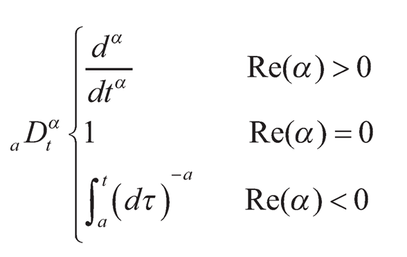 (10.1)
where a and t are the lower limit and upper limit of the integral, respectively, and a is the fractional order, which will be taken as a real number afterwards. If α > 0, a Dαt is a fractional-order differential, and if α < 0, aDαt is a fractional-order integral. Note that when the infinitesimal increment h in time equals t–a, both the left and right subscripts of the D operator can be omitted, and when a is an integer, the operator functions as the commonly seen integer D operator, that is, Dk= dk/dtk (k∈N) as a k-th order differentiator, and D -1 = ∫dτ for the first order integral and D–k =∫∫…∫dτ..dτdτ (k times k∈N) for the k-th order integral.
One most used fractional-order differential definition is the Grünwald-Letnikov definition [7], which is expressed as follows:
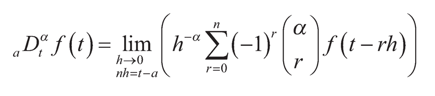 (10.2)
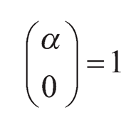
where
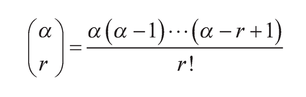 (10.3)
with
Meanwhile a famous fractional-order integral definition is the Riemann-Liouville definition [7], which is expressed as follows:
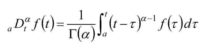 (10.4)
where
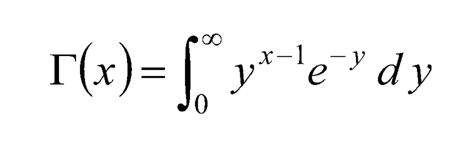 (10.5)
is the well-known Euler’s gamma function.
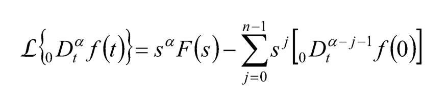
As engineering problems described by ordinary differential equations in integer order can be solved using the Laplace transform, so are those systems in fractional-order differo-integral equations.
According to the Riemann-Liouville definition, the Laplace transform for fractional-order differo-integrals is:
 (10.6)
when (n–1) ≤ α < n If 0Dt α–j–1 f (0) = 0, j= 0, 1, 2,…, n–1, then ℒ{0Dαtf(t)}= saF(s)
Now the order of the Laplace operator s is a fraction in fractional-order differo-integral.
10.2.2 PID CONTROLLERS AND ZIEGLER-NICHOLS METHOD
10.2.2.1 Pid Controllers
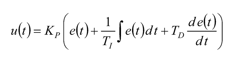
PID controllers have been popularly used after its debut. Its control effort u(t) in time domain can be expressed as:
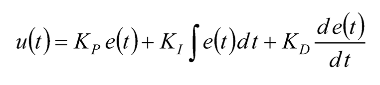 (10.7)
where Kp, Kl and KD are the proportional gain, the integral gain, and the derivative gain, respectively. And the corresponding transfer function obtained by taking the Laplace transform of Eq. (10.7) is:
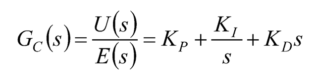 (10.8)
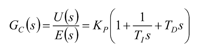
Alternatively, the parameter set is defined somehow in a different way as follows:
 (10.9)
And the corresponding transfer function of Eq. (10.9) is:
 (10.10)
By comparison of these two expressions, it is easy to conclude that K1 = Kp/T1 , and KD= KPTD. Furthermore, it’s noteworthy that the 3 terms inside the parenthesis of Eq. (10.9) have the same dimension of e(t), where the unit of T1 and TD (both of physical quantity “time”) is “second” used to cancel the unit of “dt” in the integral and derivative, respectively.
10.2.2.2 Ziegler-Nichols Method
The Ziegler-Nichols method [2] is a heuristic method for tuning PID controllers. It is meant to make the closed-loop control system’s response acceptable though not optimal. The procedure of the Ziegler-Nichols method is first to set the integral gain and derivative gain to zero which results in a P controller. Then vary the proportional gain to yield a sustained periodic oscillation in the output (or close to it) by trial and error. Mark the critical gain as the ultimate gain Ku and the corresponding period as the ultimate period Tu. Then, according to the Ziegler-Nichols method, the empirical PID parameters are assigned to be Kp= 0.6Ku , TI= Tu/2 , and TD=Tu/ 8, which is equivalent to have the alternative parameter set: Kp= 0.6Ku , KI= 1.2Ku/Tu , and KD = 3KuTu/40.
10.2.3 FRACTIONAL-ORDER PID CONTROLLERS AND TUNING RULE
10.2.3.1 FRACTIONAL-ORDER PID CONTROLLERS
Oustalop [8] proposes to apply fractional-order controllers to dynamic systems, and names such robust controllers as “Commande Robuste d’Ordre Non-Entier” (CRONE). He also introduces the fractional-order PID controller, or the PIλDμ controller (λ and μ are non-negative fractions). Similar to the PID controllers, the control effort of the fractional-order PID controller u(t) in the time domain can be expressed as:
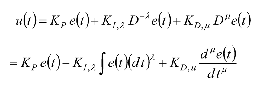 (10.11)
where Kp, KI, X, and KD,μ are the proportional gain, the fractional-order integral gain, and the fractional-order derivative gain, respectively.
And the corresponding transfer function takes the following formml:
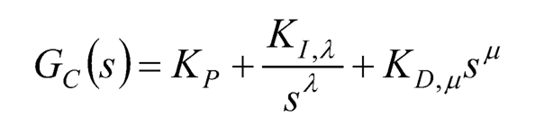 (10.12)
when λ= μ = 1 in Eq. (10.12), GC(s) is an integer PID controller; λ = 1, μ = 0, GC(s) an integer PD controller; λ = 0, μ = 1, GC(s) an integer PI controller; and λ = μ = 0, GC(s) an integer P controller. Without limiting λ and μ to be 0 or 1, the fractional-order differo-integral offers more flexibility than the integer-order differo-integral in the controller design.
10.2.3.2 TUNING RULE: GENERALIZED ZIEGLER-NICHOLS METHOD
It is desired to find a general tuning rule, just like the Ziegler-Nichols method, of setting empirical values for fractional-order PID controllers’ parameters. As mentioned in Section 10.2.2.1, the three terms inside the parenthesis of Eq. (10.9) are of the same dimension, i.e., the unit of TI and TD cancels the unit of “dt” in the integral and derivative, respectively. Keeping this in mind, now the orders of the fractional integral and derivative are λ and μ in Eq. (10.11), respectively. In order to cancel the unit of “(dt) λ” in the integral and “(dt) μ “ in the derivative, (TI) and (TD) μ can be employed in the control law for the fractional integral and derivative, respectively. Therefore, the control law for the fractional PID controller can be expressed as:
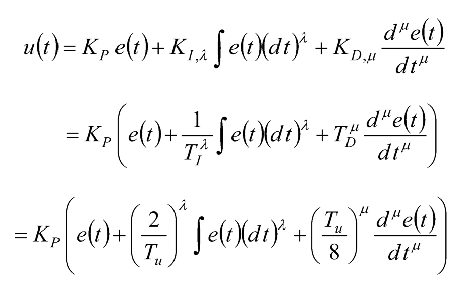 (10.13)
which yields 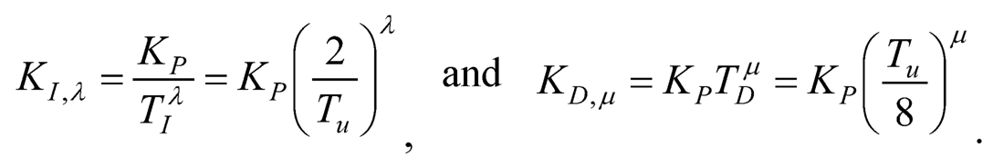
Note that λ = μ = 1 is a special case of the fractional-order PID controller, and indeed it becomes the commonly seen PID controller with parameters set by the Ziegler-Nichols method. Hence Eq. (10.13) generalizes the integer-order PID controller where λ = μ = 1.
10.2.4 IMPLEMENTATION OF FRACTIONAL-ORDER PID CONTROLLERS
10.2.4.1 APPROXIMATION OF FRACTIONAL-ORDER LAPLACE OPERATOR
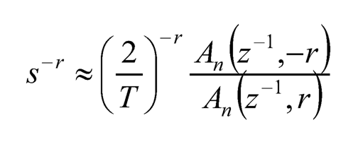
The fractional-order differentiator sr (r is a positive fraction) in continuous-time domain can be expressed in terms of z–1 in discrete-time domain by a generating function s = w(z–1) just like the integer-order differentiator s (z is an operator in Z transform); similarly it applies to the fractional-order integrator s–r (r is a positive fraction). Adopting the Tustin generating function, the fractional differo-integral would be discretized as [9]:
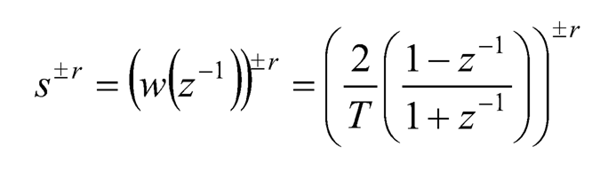 (10.14)
where 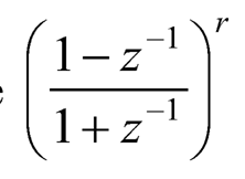 can be expanded in Taylor series as follows:
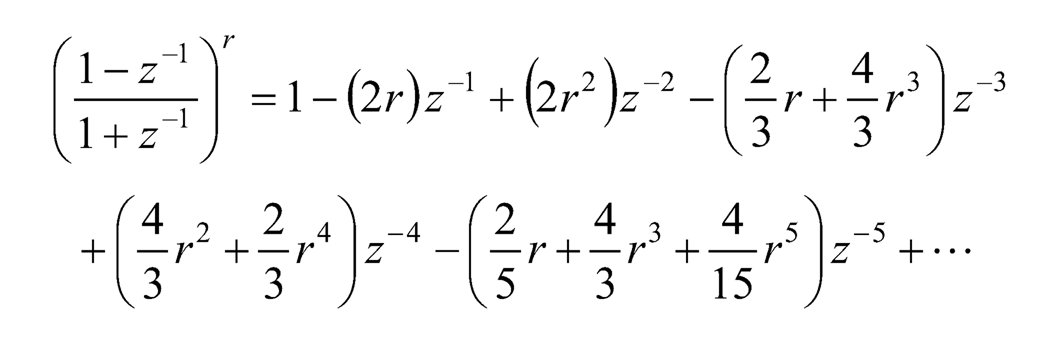 (10.15)
Therefore,
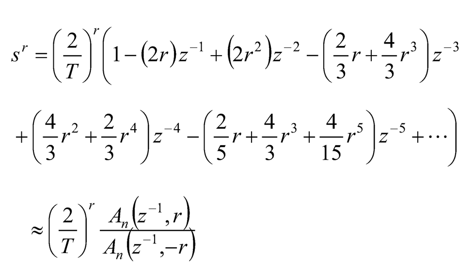 (10.16)
and
 (10.17)
where An (z–1, r), and likewise An (z–1, –r), can be found by the following iterations:
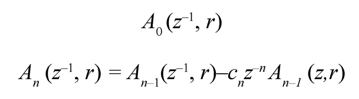 (10.18)
with the coefficient: 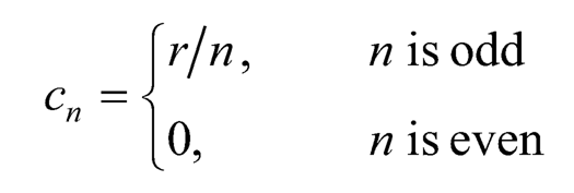
Without doubt the accuracy of the approximation is determined by the selection of n.
10.2.4.2 IMPLEMENTATION OF FRACTIONAL-ORDER PID CONTROLLERS
By substituting the above discrete-time approximation of the fractional-order Laplace operator sr and s–r into Eq. (10.11), the fractional-order PID controller in Eq. (10.10) can be approximated in discrete-time domain as:
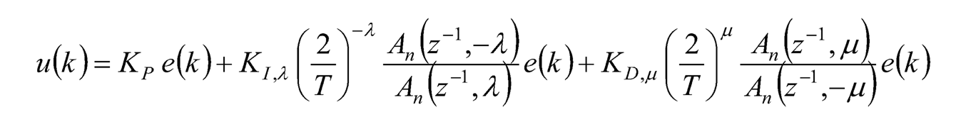 (10.19)
where the index k stands for the k-th sampling time, e.g., e(k)= e(t = kTs) with sampling time Ts.
10.3 AN UNDERACTUATED SYSTEMML: A ROTARY PENDULUM SYSTEM
A rotary pendulum system (Figure 10.1) which uses a permanent magnet DC motor to drive a two-link rotary pendulum is the underactuated system employed to demonstrate the performance of the fractional-order PID controller in this research. The rotary pendulum system is an underactuated system because there is only one actuator to drive link 1 but no actuator to drive link 2. Both links have one rotational degree of freedom (d.o.f.) around different axes. The motion of link 2 is coupled with link 1 so it has to be considered when controlling link 1.
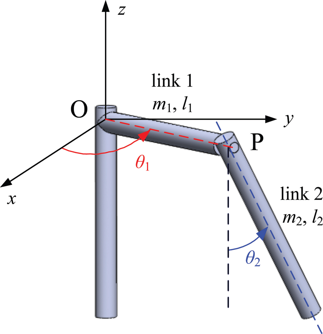
FIGURE 10.1 The two-link rotary pendulum.
10.3.1 DC MOTOR MODEL
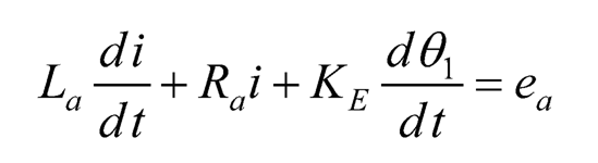
A DC motor model is used to drive the two-link rotary pendulum. The armature voltage is ea, and the current through the armature is i. The armature current generates a motor torque τM= KTi, where KT is the torque constant of the DC motor. Assume that the angular displacement of the motor shaft is θ and the load is τL, then the mechanical dynamics of the DC motor is:
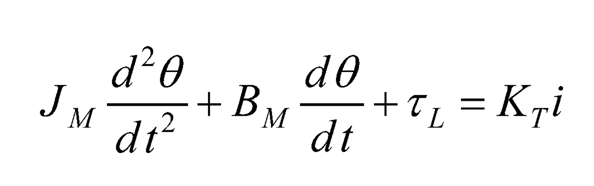 (10.20)
where JM and BM are the rotational inertia and the rotational damping coefficient of the motor, respectively.
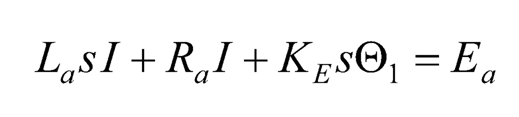
As the motor shaft rotates at a speed ω = dθ/dt, the so-called back e.m.f. is induced by the relationship eb.e.m.f. = KEω where KE is the back e.m.f. constant of the DC motor and KE = KT in the SI unit system. Then applying the Kirchhoff’s voltage law to the armature gives the electrical dynamics of the DC motor below:
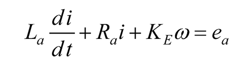 (10.21)
where La and Ra are the inductance and resistance of the armature, respectively.
10.3.2 TWO-LINK ROTARY PENDULUM MODEL
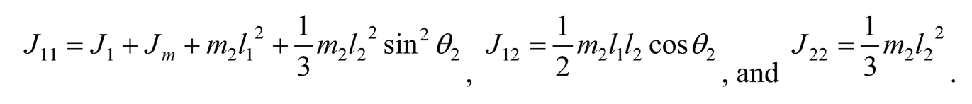
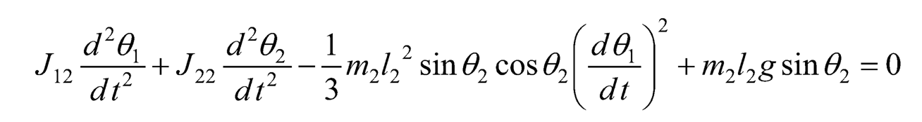
The mechanical part of the rotary pendulum, driven by the torque τL, consists of two rotational links of 1 d.o.f. each: link 1 and link 2 as shown in Figure 10.1. Link 1 is connected to the motor shaft and rotates around the center O, and link 2 is connected to the other end of link 1 and rotates around point P in a plane normal to link 1. The masses of link 1 and 2 are m1 and m2, respectively. The lengths of link 1 and 2 are l1 and l2, respectively. And the moment of inertia of link 1 around O is J1. Assume that θ1 and θ2 are the angular displacements of link 1 and 2, respectively. Then the angular velocities of link 1 and 2 are θ̇̇1and θ̇̇2 respectively. Since the center O is on the motor shaft, it is straightforward θ1 = θ.
The dynamic model of the two-link rotary pendulum can be derived using the Euler-Lagrange equation [10]:
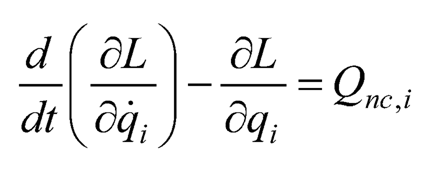 (10.22)
where the Lagrangian L is the difference of the kinetic energy T and potential energy V of the system (L = T – V), qi is the i-th generalized coordinate, and Qnc,i is the i-th non-conservative generalized force. The kinetic energy is:
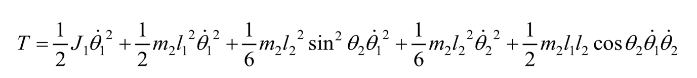 (10.23)
where only the first term accounts for link 1, and the other 4 terms are from link 2. Meanwhile, the potential energy only comes from link 2, which is:
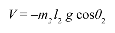 (10.24)
Therefore the Lagrangian is:
 (10.25)
where θ1 and θ̱̱2are chosen as the 2 generalized coordinates, then the corresponding Euler-Lagrange equations are:
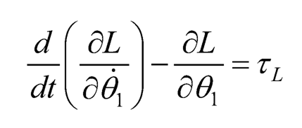 (10.26)
and
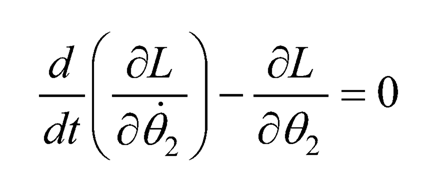 (10.27)
The dynamic equation of the mechanical subsystem then can be expressed as follows:
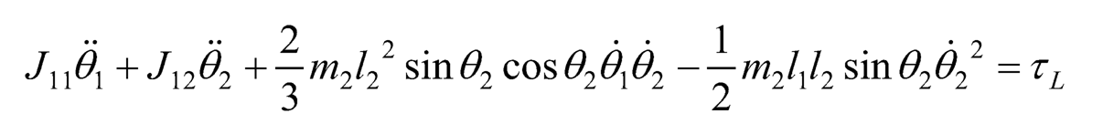 (10.28)
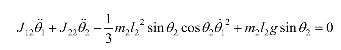 (10.29)
where
10.3.3 COMPLETE SYSTEM MODEL
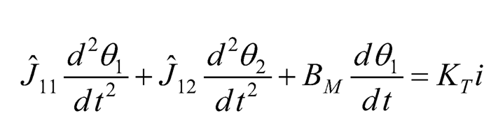
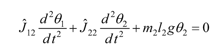
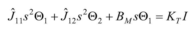
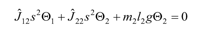
The complete system consists of a DC motor represented by Eq. (10.20) and (10.21), and a two-link rotary pendulum represented by Eq. (10.28) and (10.29). Since Eq. (10.28) gives the term τL, it can be substituted into Eq. (10.20), and using the fact that θ1 = θ, then the whole system therewith can be represented by the dynamic model below.
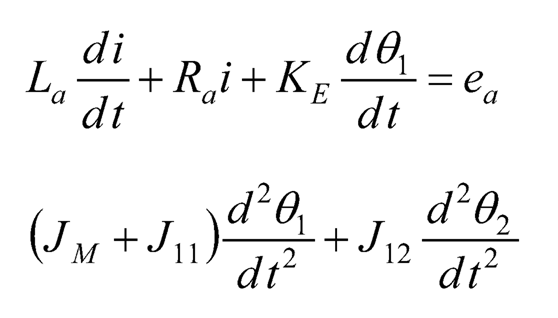 (10.30)
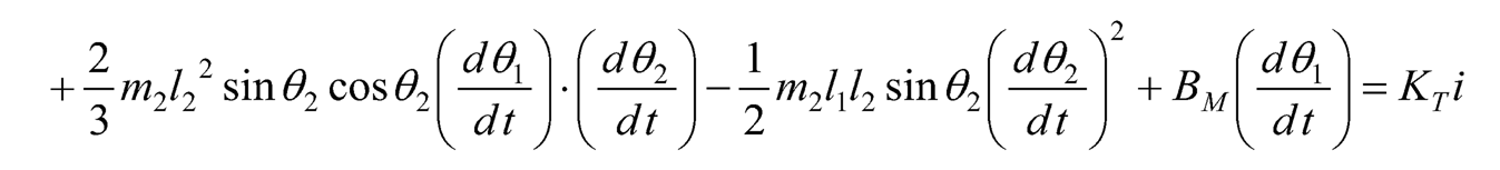 (10.31)
 (10.32)
10.4 ESTIMATION OF CONTROLLER PARAMETERS
The aforementioned fractional-order Laplace operator approximation is used to design the fractional-order PID controller for the rotary pendulum system, and the proposed fractional-order Ziegler-Nichols method is employed to tune parameters. Then the results will be compared with the result of using the traditional Ziegler-Nichols method tuned integer-order PID controller. One important step of the Ziegler-Nichols method is to find the ultimate gain Ku and the corresponding period Tu for consistent oscillation. However, the trial-and-error approach would be time-consuming; it is desired to have the theoretical groundwork to make a reasonable estimation of Ku to save trouble.
The Ruth-Hurwitz stability criterion [11] can be used to find the ultimate gain Ku in a linear system. Since the rotary pendulum system is nonlinear, it helps if the local linearization method is used to linearize the system around an operating point before using the Ruth-Hurwitz stability criterion to find the ultimate gain Ku. The approach will be detailed in this section.
10.4.1 LOCAL LINEARIZATION OF THE TWO-LINK ROTARY PENDULUM SYSTEM
The equilibrium point of the rotary pendulum, i.e., θ2 = 0, is chosen to be the operating point for local linearization. First assume that θ2≈ 0. Next linearize the dynamic Eqs. (10.31)–(10.32) by using the approximation sin θ2≈ θ2, cos θ2 ≈ 1, θ2 ≈ 0, and at equilibrium, then setting the higher order terms to zeros. Hence, the linearized model of the rotary pendulum can be expressed as:
 (10.33)
 (10.34)
 (10.35)
where Ĵ11=JM+J1+m2l12, Ĵ12=1/2m2l1l2 Ĵ22=1/3m2l22
Taking the Laplace transform of Eqs. (10.33)–(10.35) yields the following system of equations:
 (10.36)
 (10.37)
 (10.38)
Since Eq. (10.38) contains only two unknowns Θ1 and Θ2, Θ2 can be expressed in terms of Θ1 as:
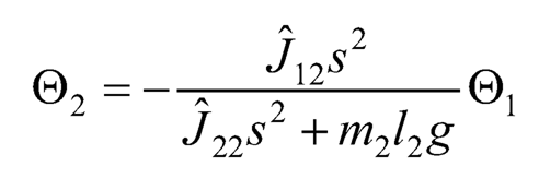 (10.39)
By substituting the result into Eq. (10.37), Θ1 can be expressed in terms of I as:
 (10.40)
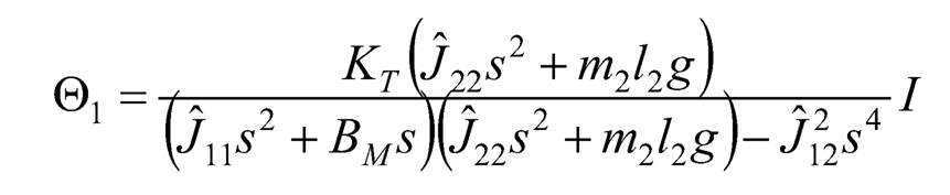
and the transfer function of link 1’s angular displacement to armature current is:
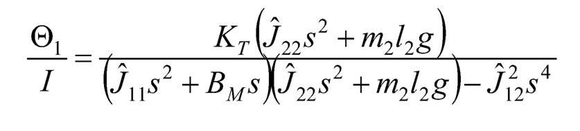 (10.41)
Alternatively, Eq. (10.40) can be rewritten in a different way as:
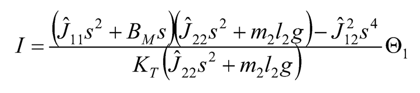 (10.42)
Then by substituting Eq. (10.42) into Eq. (10.36), Θ1 can be expressed in terms of Ea as:
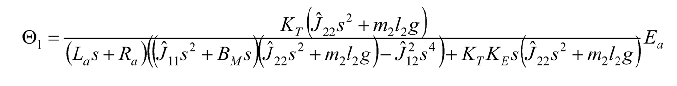 (10.43)
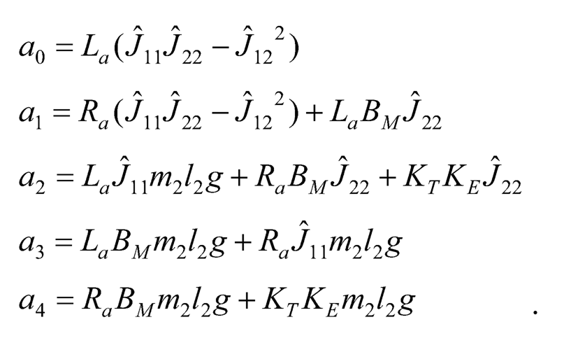
And the transfer function of link 1’s angular displacement to armature voltage can be expressed as:
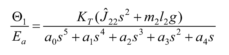 (10.44)
where
10.4.2 TRANSFER FUNCTION OF THE CLOSED-LOOP CONTROLLED ROTARY PENDULUM SYSTEM
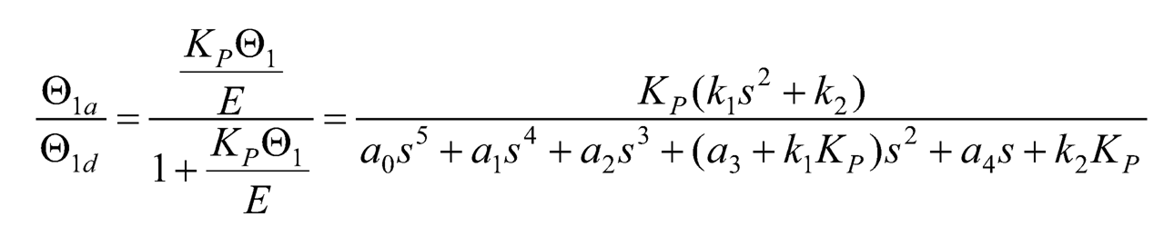
Figure 10.2 shows the block diagram of a typical closed-loop control system. The plant is the DC motor-driven rotary pendulum system, the reference input r is the desired link 1’s angular displacement input θ1d, the system output y is the actual link 1’s angular displacement output θ1a, and the control effort u is the armature voltage ea in this research. When using a P controller with gain Kp to control the rotary pendulum system, the closed-loop transfer function of the actual angular displacement output θ1a to the desired angular displacement input O1d becomes:
 (10.45)
where k1= KT J22 and k2= KT m2l2g. And its characteristic equation is:
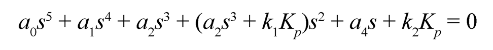 (10.46)
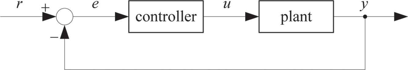
FIGURE 10.2 Block diagram of a closed-loop control system.
10.4.3 ESTIMATION OF THE ULTIMATE GAIN USING THE RUTH TABLE
The following DC motor parameters and two-link rotary pendulum parameters are used: La = 4.6909 × 10⁻³, Ra = 2.5604 Ω, KT = 1.8259 × 10⁻² N·m/A, KF = 1.8259 ×10⁻² V/(rad/s), JM = 7.2019 × 10⁻⁵ kg·m2, BM = 9.1358 × 10⁻⁵ N·m(rad/s), m1 0.056 kg, l1 = 0.16 m, J1 0.001569 kg·m2, m2 = 0.022kg, and l2 = 0.16m. The coefficients of the characteristic equation calculated are a0 ≈ 1.5691 × 10⁻⁹, a1 ≈ 8.5655 × 10⁻⁷, a2 ≈ 4.6355 × 10⁻⁷, a3 ≈ 1.949 × 10⁻⁴, a4 ≈ 1.959 × 10⁻⁵, k1 ≈ 3.4278 × 10⁻⁶, and k2 ≈ 6.3051 × 10⁻⁴. And the Ruth table [11] is shown in Table 10.1.
TABLE 10.1 Ruth Table with KP as a Variable
| S5 | 1.5691 × 10⁻⁹ | 4.6355 × 10⁻⁷ | 1.959 × 10⁻⁵ |
| s4 | 8.5655 × 10⁻⁷ | (1.949 × 10⁻⁴ + 3.4278 × 10⁻⁶Kp ) | 6.3051 × 10⁻⁴KP |
| s3 | A1 | A2 | – |
| s2 | B1 | 6.3051 × 10⁻⁴KP | – |
| s1 | C1 | – | |
| s0 | 6.3051 × 10⁻⁴Kp | – | – |
There are three cases in determining the ultimate gain Ku: (1) A1 = 0, (2) B1 = 0, and (3) C1 = 0. However, only the third case gives a reasonable solution. For the third case, i.e., C1 = 0 or the first term in the s1 row is zero, KP ≈ 16.9592 is found which gives A1 > 0, B1 > 0, and is chosen as the ultimate gain Ku. (The corresponding Ruth table is shown in Table 10.2.) Though the ultimate gain Ku ≈ 16.9592 is calculated using the linearized model, not the actual nonlinear model, it’s good to choose it as an initial guess to find the closest Ku and Tu, and therewith determine the corresponding controller parameters (which will be given in the next section) to complete the controller design.
TABLE 10.2 Ruth Table with Kp ≈ 16.9592
| s5 | 1.5691 × 10⁻⁹ | 4.6355 ×10⁻⁷ | 1.959 × 10⁻⁵ |
| s4 | 8.5655 × 10⁻⁷ | 2.5303 × 10⁻⁴ | 0.0107 |
| s3 | 1.2805 × 10⁻¹¹ | 6.3217 × 10⁻¹⁰ | – |
| s2 | 2.1075 × 10⁻⁴ | 0.0107 | – |
| s1 | 0 | – | |
| s0 | 0.0107 | – | – |
10.5 SIMULATION RESULTS
This research will evaluate the fractional-order PID controller’s performance by simulation in this section. The point-to-point maneuver is the task. To maneuver a system to a target position, step input is often used in textbooks to evaluate the controller’s performance by the response. It’s also used traditionally in the Ziegler-Nichols method in determining the PID parameters. Yet trajectory planning makes the transition smoother and is practically used in motion control. Trapezoidal curve (T curve) and sigmoid curve (S curve) are two popularly used speed profiles in trajectory planning. For simplicity and demonstration purpose, a symmetric T-curve speed profile is adopted as &θ1d to generate the desired link 1’s angular displacement trajectory O1d (as shown in Figure 10.2). And the planned trajectory serves for finding the ultimate gain Ku and the ultimate period Tu using Ziegler-Nichols method, and evaluating the performance of the tuned PID controller and fractional-order PID controllers of 3 different fractions in this section.
10.5.1 TRAJECTORY PLANNING
A symmetric T-curve speed profile is adopted as the rotational speed and used for generating the desired angular displacement trajectory. Basically, it consists of one constant acceleration phase, one constant speed phase, and one constant deceleration phase. Assume the angular acceleration is am at the first phase (0 ≤ t < t1), the angular speed ωm= αmt1 at the second phase (t1 ≤ t < t2), and the angular deceleration –am at the third phase (t2 ≤ t < t3). After the third phase (t ≥ t3), the desired position stays at the target position (total angular displacement). The desired angular acceleration αd (t) = θ̈ d(t), angular speed ωd (t) = θ̈ d(t), and angular displacement θd(t) of a general symmetric T-curve angular speed (Figure 10.3) can be described as follows:
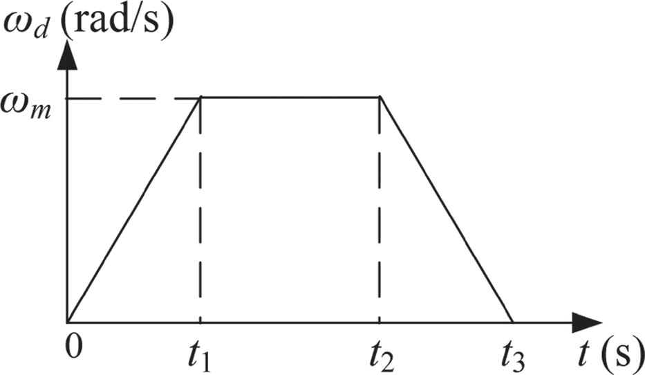
FIGURE 10.3 Trapezoidal curve angular speed profile.
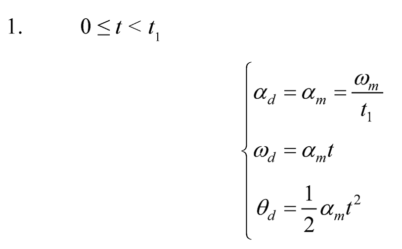 (10.47)
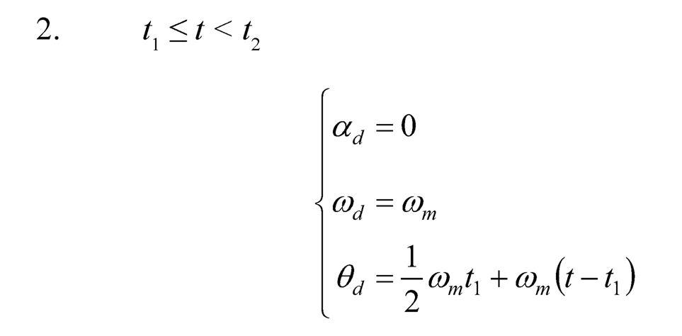 (10.48)
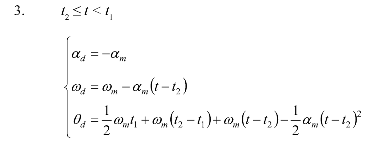 (10.49)
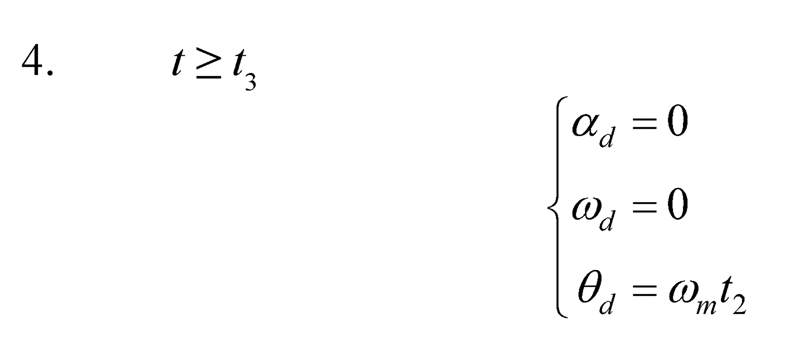 (10.50)
10.5.2 RESULTS AND DISCUSSIONS
This section presents simulation results of the DC motor-driven two-link rotary pendulum system. The parameters in Section 10.4.3 are used in this section. Initial values of θ1 = 0, θ2 = 0, θ̇1 = 0, and θ̇2 = 0 are chosen. The target link 1’s angular displacement is set to be θ1d= π/2 = 90o. Hence the T-curve angular speed profile mentioned in the previous subsection is employed to generate link 1’s trajectory with parameters θ̇1,max =π/3rad/s, t1 = 0.5 s, and t3 = 2 s.
The first step of the Ziegler-Nichols method is to set KI = 0, and KD= 0, then find the ultimate gain Ku which makes the closed-loop system have consistent oscillation in the output. As suggested in Section 10.4.3, the theoretical value Ku ≈ 16.9592 calculated from the Ruth table built for the linearized model is used as an initial guess to find the ultimate gain of the actual nonlinear model. Within a few trials, it is found that the closed-loop system have consistent oscillation in the output when Kp= 16.96 as shown in Figure 10.4, hence the ultimate gain Ku is chosen to be 16.96. Also, the ultimate period Tu is about 0.80736 s as seen in Figure 10.4.
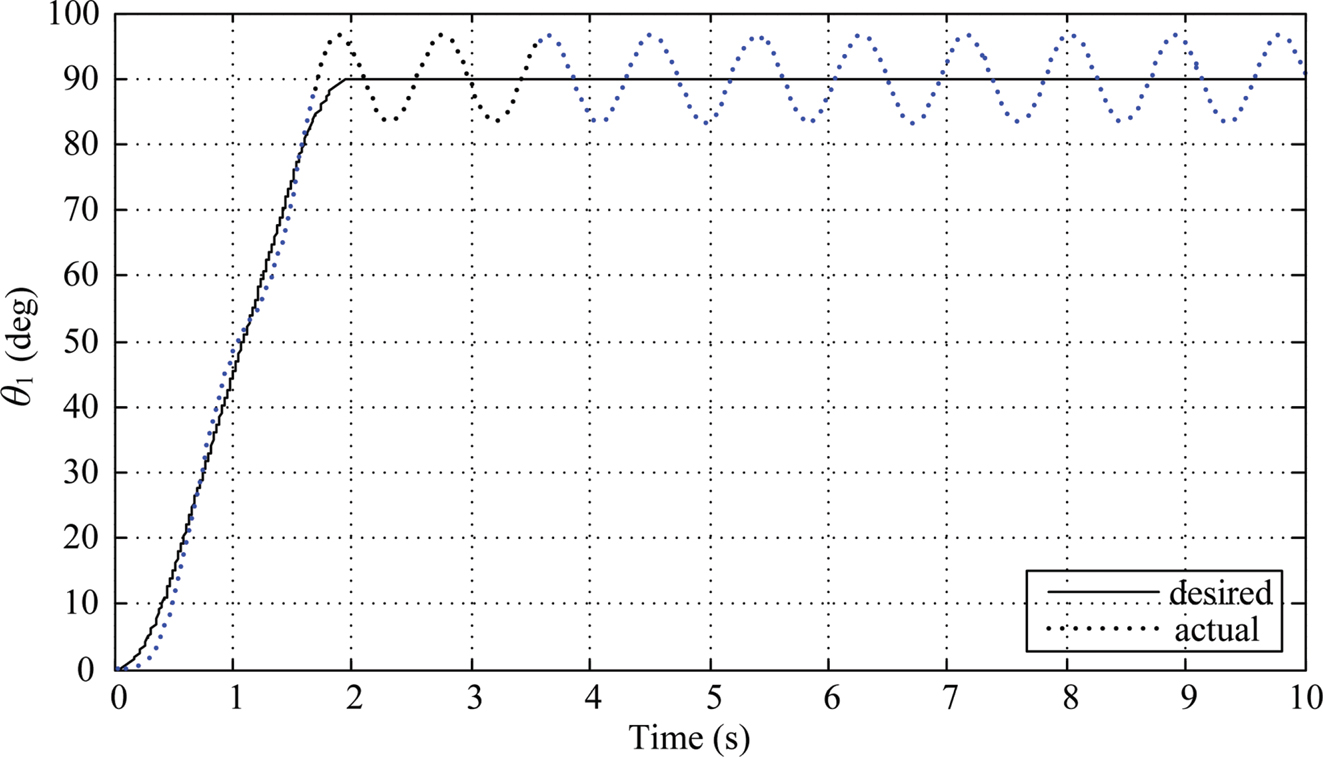
FIGURE 10.4 Link 1’s response under P control (Kp = 16.96, KI= 0, KD = 0).
According to the Ziegler-Nichols method, choose the PID parameters to be Kp= 10.176, KI = 25.2081, and KD = 1.02696. The simulation results using the tuned PID parameters show that the maximum overshoot of link 1 is 5.135o, and the settling time for the settling window of ±5% (± 4.5o for 90o motion) occurs at ts = 2.163s (0.163 s after the 2-second T-curve motion) as shown in Figure 10.5. There is a trend of 1/4 decay oscillation after 2 s. The maximum swing angle of link 2 is θ2≈ –1.7o (Figure 10.6). And the time history of the control armature voltage is shown in Figure 10.7. The armature voltage also shows 1/4 decay oscillation after 2 s just like Figure 10.5.
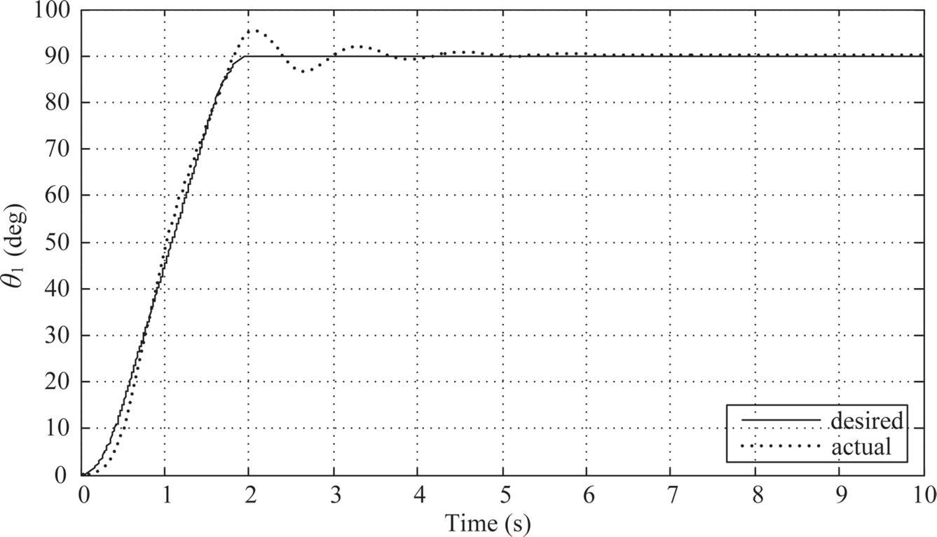
FIGURE 10.5 Link 1’s response under PID control (KP = 10.176, KI = 25.2081, KD = 1.02696).
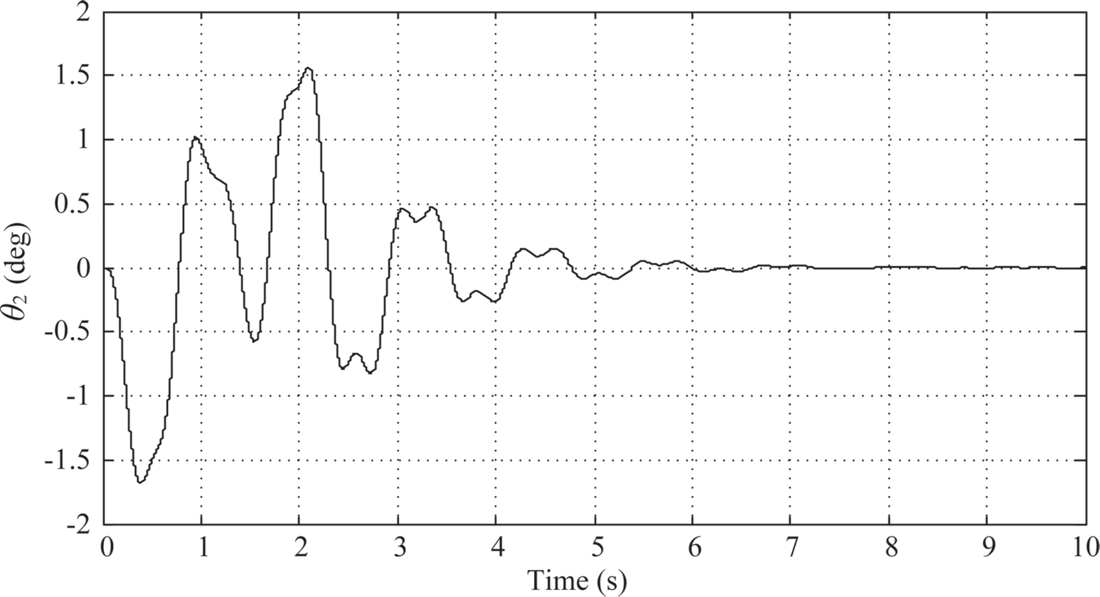
FIGURE 10.6 Link 2’s response under PID control (KP = 10.176, KI = 25.2081, KD = 1.02696).
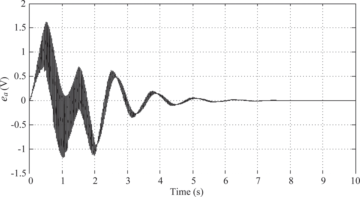
FIGURE 10.7 Armature voltage under PID control (KP = 10.176, KI = 25.2081, KD = 1.02696).
Next the fractional-order PID control will be employed so as to make comparison with the tuned (intger order) PID control. As proposed in Subsection 10.2.2.2, KP = 0.6Ku, KIλ = KP / TIλ = KP (2 / Tu)λ, and KD,µ = KPTDμ = KP (Tu / 8)μ are used for the fractional integral gain and the fractional derivative gain, respectively. Though the output θ1 and the internal state θ2 are coupled, there is a certain relationship between them. It would be straightforward to choose λ = μ then. Three sets of fractional-order PID parameters are used for comparison: (1) λ = μ = 0.4, (2) λ = μ = 0.5, and (3) λ = μ = 0.6. Here are the results:
1. λ = μ = 0.4: The controller parameters are chosen to be KP = 10.176, KI,λ≈ 14.62723, and KD, μ ≈ 4.0660. As shown in Figure 10.8, the maximum overshoot of link 1 is about 0.71o and the actual angular displacement of link 1 stays within the settling window after the planned 2-sec. moving time.
The maximum swing angle of link 2 is around –2.9o (Figure 10.9). And the time history of the control armature voltage is shown in Figure 10.10. However, there is no sign of decay after 2 s. After 2 s, Link 1 and link 2 are oscillating between ±1o and ±1.3o, respectively, and the armature voltage is oscillating between ±0.4o (V).

FIGURE 10.8 Link 1’s response under PIλDμ control (λ = μ = 0.4).
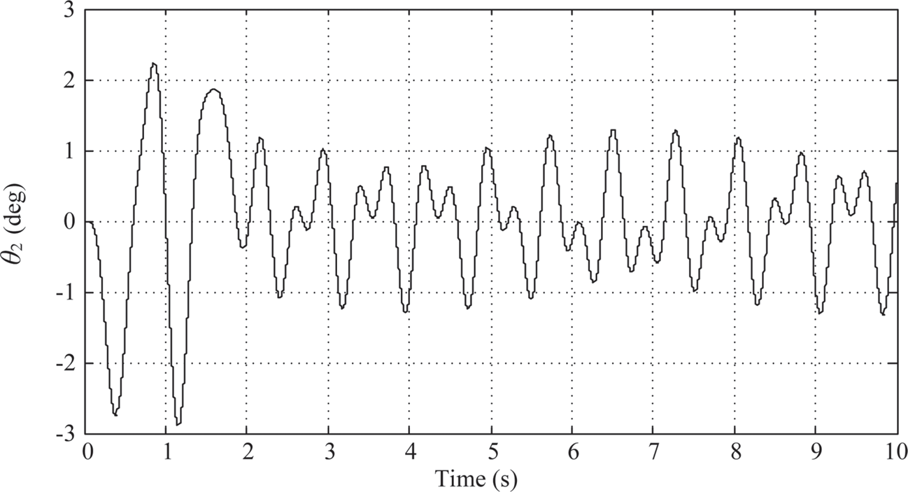
FIGURE 10.9 Link 2’s response under PIλDμ control (λ = μ = 0.4).
2. λ = μ = 0.5: The controller parameters are chosen to be KP = 10.176, KI,λ≈ 16.01616, and KD, μ ≈ 3.2327. As shown in Figure 10.11, the maximum overshoot of link 1 is about 0.15o and the actual angular displacement of link 1 stays within the settling window after the planned 2-sec. moving time.
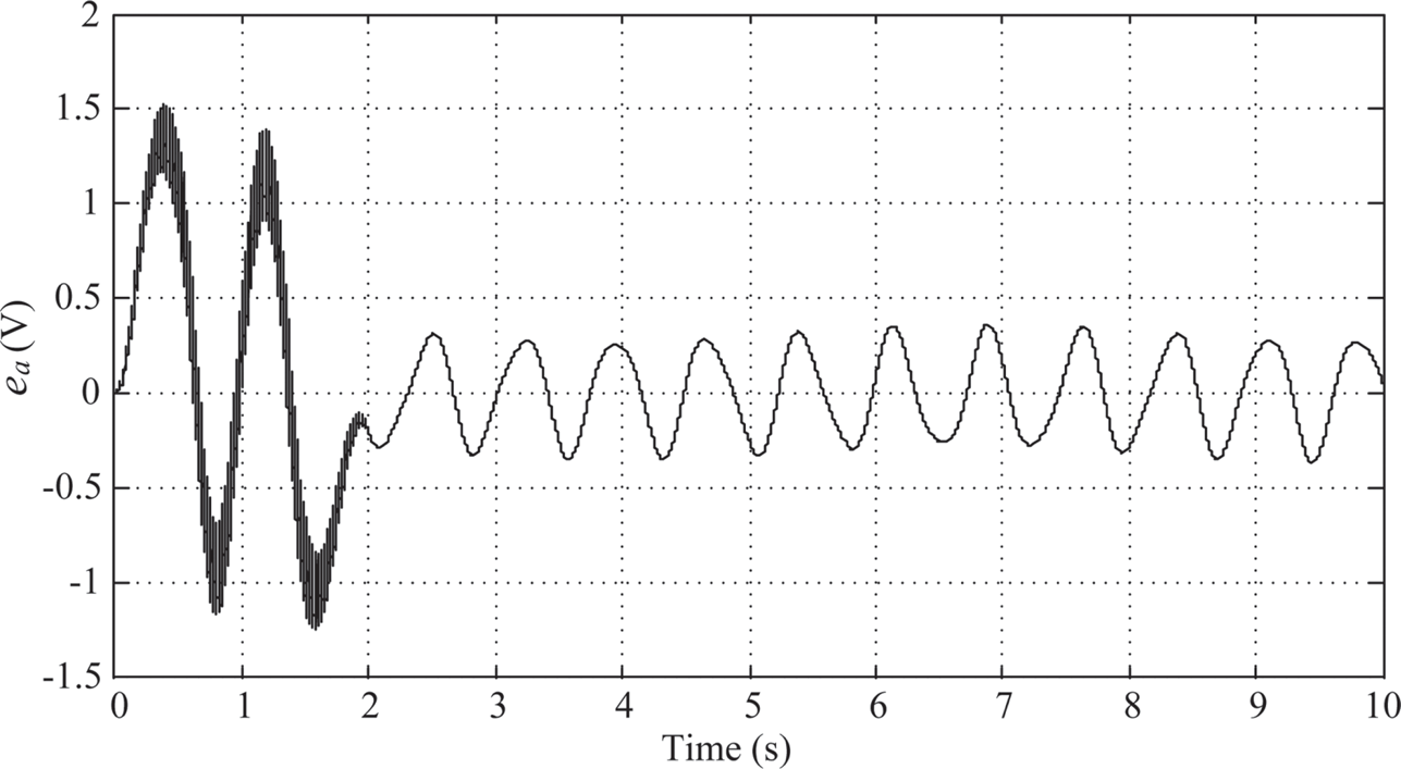
FIGURE 10.10 Armature voltage under PIλDμ control (λ = μ = 0.4).
The maximum swing angle of link 2 is around –2.8o (Figure 10.12). And the time history of the control armature voltage is shown in Figure 10.13. Again, there is no sign of decay after 2 s. After 2 s, Link 1 and link 2 are oscillating between ± 0.5o and ± 0.8o, respectively, and the armature voltage is oscillating between ± 0.15(V).
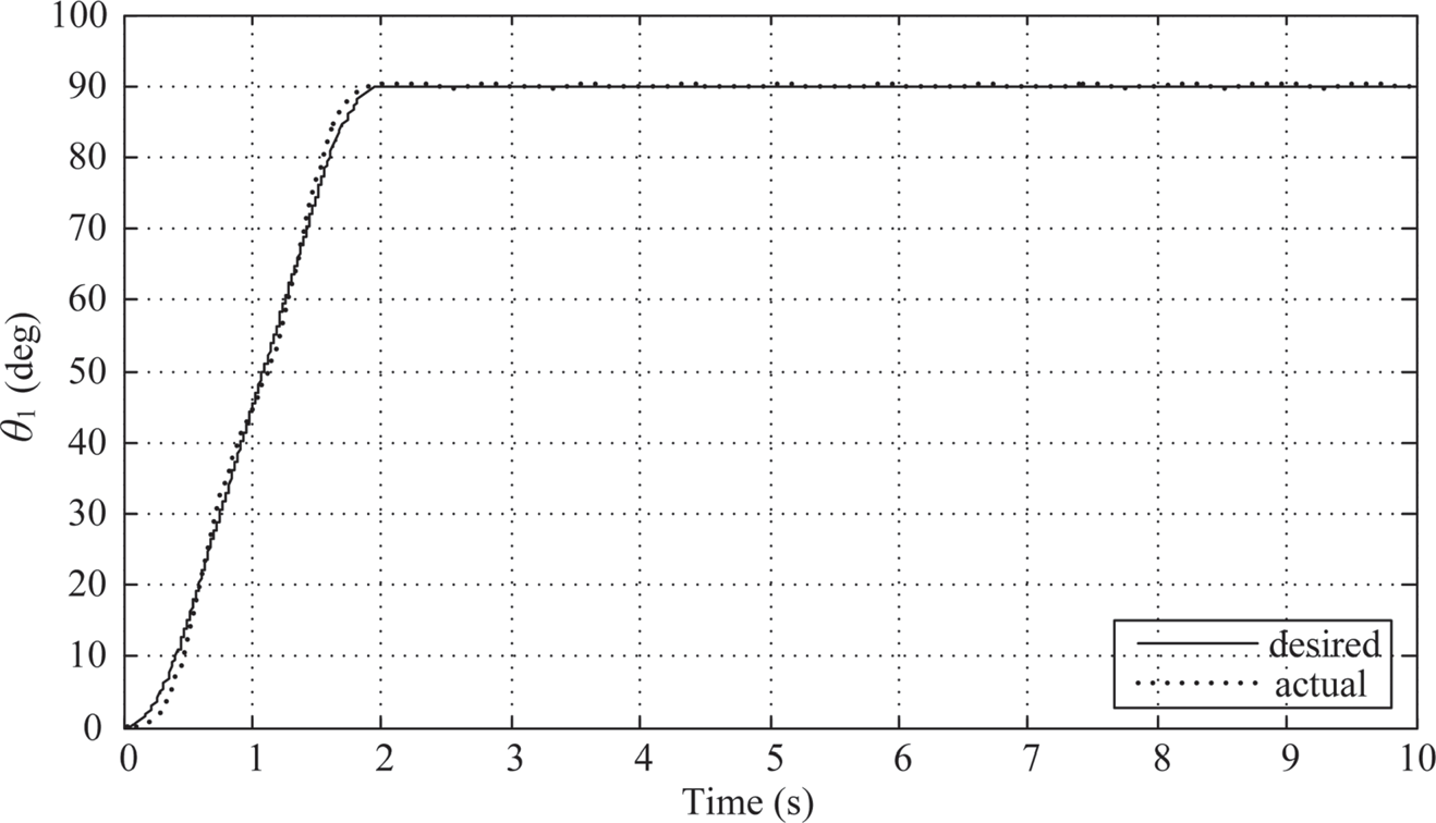
FIGURE 10.11 Link 1’s response under PIλDμ control (λ = μ = 0.5).
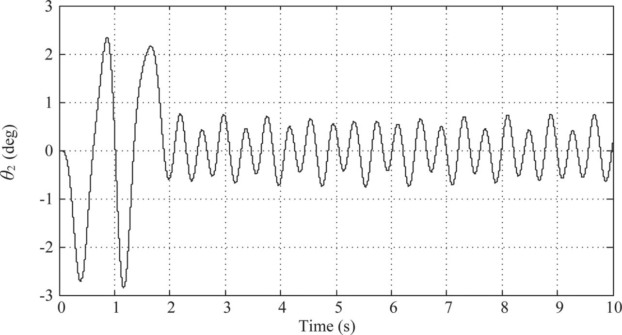
FIGURE 10.12 Link 2’s response under PIλDμ control (λ = μ = 0.5).
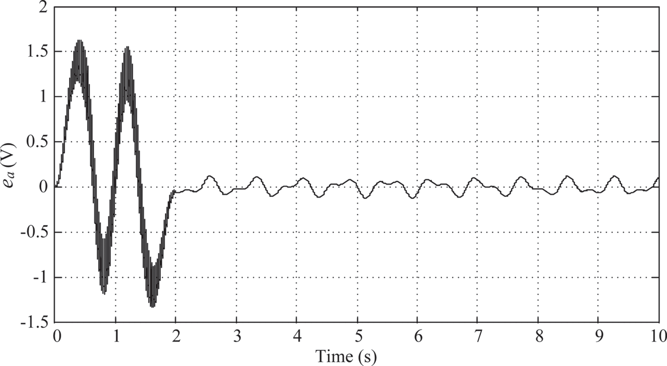
FIGURE 10.13 Armature voltage under PIλDμ control (λ = μ = 0.5).
3. λ = μ = 0.6: The controller parameters are chosen to be KP = 10.176, KI, λ ≈ 17.53698, and KD, μ ≈ 2.57018. As shown in Figure 10.14, the maximum overshoot of link 1 is about 0.4o and the actual angular displacement of link 1 stays within the settling window after the planned 2-sec. moving time.
The maximum swing angle of link 2 is around –2.8o(Figure 10.15). And the time history of the control armature voltage is shown in Figure 10.16. However, there is no sign of decay after 2 s. After 2 s, Link 1 and link 2 are oscillating between ± 1o and ± 0.9o, respectively, and the armature voltage is oscillating between ± 0.2 (V).

FIGURE 10.14 Link 1’s response under PIλDμ control (λ = μ = 0.6).
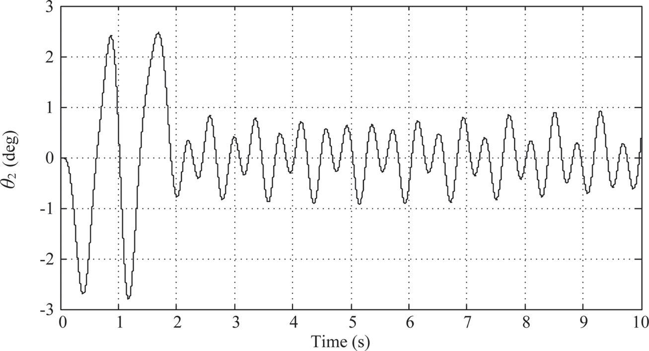
FIGURE 10.15 Link 2’s response under PIλDμ control (λ =μ = 0.6).
Generally speaking, the performance of all three fractional-order PID controllers, designed using the proposed generalized Ziegler-Nichols method, is better than that of the integer-order PID controller, designed using the Ziegler-Nichols method in terms of tracking during 2-sec. motion, overshoot, and settling time. However, oscillation continues even after 10 sec. if any of these three fractional-order PID controllers is used, while oscillation decays to zero if the integer-order PID controller is used. This might suggest that the proposed generalized Ziegler-Nichols method should be further improved in order to have the system converges to zero.
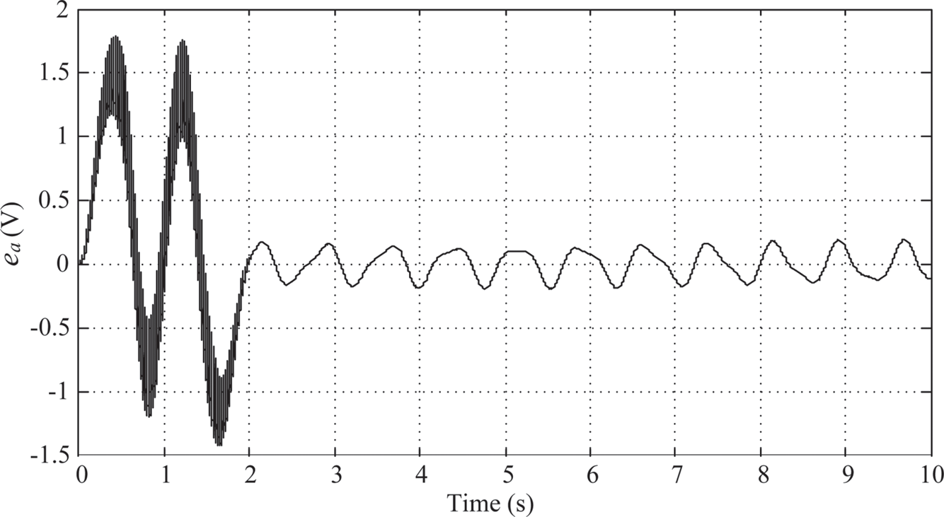
FIGURE 10.16 Armature voltage under PIλDμ control (λ = μ = 0.6).
Now among these three fractional-order PID controllers, the one comes with λ = μ = 0.5 shows the best performance in every way which implies the system is more likely to have fractional order 0.5 than 0.4 or 0.6.
10.6 CONCLUSIONS
The performance of the tuned PID controller and three tuned PIλDμ controllers are compared when applied to control an underactuated system. The use of local linearization and Ruth-Hurwitz stability criterion gives a very close approximation of the ultimate gain for the actual nonlinear system. It seems that λ and μ should be equal based on the order of the coupled dynamics of link 1 and link 2. A generalized Ziegler-Nichols method for the fractional-order PID controller is proposed to include the integer-order PID controller as a special case λ = μ = 1. It keeps the simplicity of the Ziegler-Nichols method. The simulation results show that the system is more likely to have fractional order 0.5 than 0.4 or 0.6 based on their performance. Meanwhile, these three tuned PIλDμ controllers work better in terms of tracking during 2-sec. motion, overshoot, and settling time, especially settling time, but not oscillation decay rate. Yet these results show the fractional-order controller is promising if the oscillation problem can be dissolved. Hence more vigorous researches should be conducted to improve the proposed generalized Ziegler-Nichols method so it can be used in versatile control applications.
KEYWORDS
• Commande Robuste d’Ordre Non-Entier
• fractional-order
• parameter tuning
• trajectory planning
• underactuated system
• Ziegler-Nichols method
REFERENCES
1. Miller, K. S., & Ross, B., (1993). An Introduction to the Fractional Calculus and Fractional Differential Equations. Wiley: New York.
2. Ziegler, J. G., & Nichols, N., (1942). Optimum settings for automatic controllers. Transactions of the ASME, 64, 759–768.
3. Monje, C. A., Vinagre, B. M., Feliu, V., & Chen, Y., (2008). Tuning and auto-tuning of fractional-order controllers for industry applications. Control Engineering Practice, 16(7), 798–812.
4. Valério, D., & Sá Da Costa, J., (2006). Tuning of fractional PID controllers with Ziegler-Nichols-type rules. Science Signal Processing, 86(10), 2771–2784.
5. Singh, A. P., Srivastava, T., Agrawal, H., & Srivastava, P., (2017). Fractional-order controller design and analysis for crane system. Progress in Fractional Differentiation and Applications, 3(2), 155–162. doi: 10.18576/pfda/030206.
6. Singh, A. P., Agarwal, H., & Srivastava, P., (2015). Fractional-order controller design for inverted pendulum on a cart system (POAC). WSEAS Transactions on Systems and Control, 10, 172–178.
7. Fan, H., Sun, Y., & Zhang, X., (2007). Research on fractional-order controller in servo press control system. IEEE International Conference on Mechatronics and Automation. Harbin, China. [Online] doi: 10.1109/ICMA.2007.4304026. https://ieeexplore.ieee.org/document/4304026 (accessed on 13 May 2020).
8. Oustaloup, (1995). La Derivation non-Entiere. Hermes: Paris, France.
9. Chen, Y. Q., & Moore, K. L., (2002). Discretization schemes for fractional-order differentiators and integrators. IEEE Transactions on Circuits and Systems I: Fundamental Theory and Applications, 49(3), 363–367.
10. Meirovitch, L., (1970). Methods of Analytical Dynamics. McGraw-Hill: New York.
11. Nise, N. S., (2015). Control Systems Engineering (7th edn.). Wiley: New York.