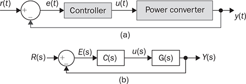
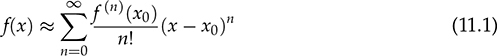
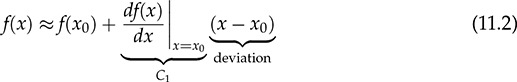
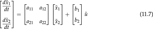
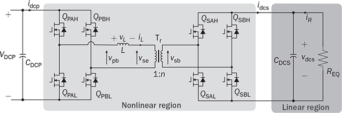
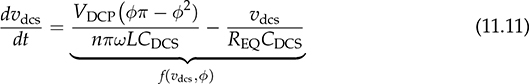
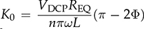
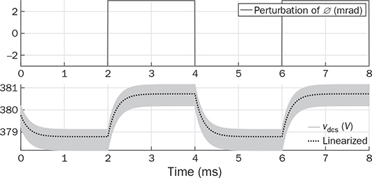
The automatic control is based on the closed-loop concept, which adopts sensing, computation, and correction. Figure 11.1a illustrates a typical feedback control system that regulates power converters. Depending on the system requirement, the control loop is commonly specified and designed to achieve one of the following functions: FIGURE 11.1 Feedback control diagram: (a) application; (b) modeled. • Voltage regulation of either input or output. • Current regulation of either input or output. • Power regulation of either input or output. Dynamic modeling is an important step to reveal the important feature of a dynamic system in terms of response speed, damping, steady state, stability, and robustness. It is considered the first step but critical for controller development. After modeling, a dynamic power system can be represented by the transfer function in the frequency domain, as illustrated in Figure 11.1b. The objective of dynamic modeling aims to find the mathematical model of G(s) to represent the key dynamics. The on/off switching of power converters is discontinuous, which cannot be directly represented by a linear model. The dynamic models of buck converters have been completely developed using averaging techniques when only the continuous conduction mode (CCM) is considered. The modeling has been described in Sec. 10.2.1 and expressed by the transfer functions in (10.8) and (10.9). The models are ready to be utilized for the dynamic analysis and feedback controller design. However, the averaging process of other topologies, e.g., boost and buck-boost, leads to the nonlinearity of differential equations, which cannot be directly applied for the linear control analysis and design. The switching between the CCM and DCM increases the modeling complexity and leads to nonlinearity. Linearization is required to derive small-signal models that can be analyzed and evaluated by the well-developed linear control theory. A function is represented by y = f(x), linear or nonlinear. If f(x) is infinitely differentiable, the Taylor series expansion regarding an equilibrium point (x0, y0) can be expressed by where n! denotes the factorial of n, and f(n)(x0) denotes the nth derivative evaluated at the point x0. The higher value of n indicates a better approximation of the function of f(x) by the Taylor series. Neglecting the higher-order terms, the first-order approximation is the simplest and expressed by (11.2) when n = 1. where C1 becomes a constant parameter showing the direction and speed. The function f(x) = f(xo) + C1(x − x0) is the approximation of the nonlinear function of f(x) near the equilibrium point (x = x0). The approximation is only valid when the deviation is not far from the equilibrium point (x0, y0). When a differential equation, A small perturbation or deviation is defined as The above operation shows the concept of linearization and represents a nonlinear system into the linearized or small-signal model. The linearized model is only valid or representative near the equilibrium point (x0, y0). The same approximation can be used for the nonlinear equations, which show multiple state variables and inputs. A simple system with two state variables (x1, x2) and one control input (u) is expressed by where f(x1, x2, u) and g(x1, x2, u) are nonlinear. The nonlinear model is representative and can be used to represent the converter dynamics. For example, the x1 can refer to the inductor current, x2 symbolizes the output voltage, and u is the duty ratio of the PWM. The values of X1, X2, and U are the state variables and control input at the equilibrium point or steady state, expressed by Applying partial differentiation, the linearized dynamics of the two state variables can be expressed by where the perturbation or small variant is indicated by “tilde” and defined by Following the linearization, the variables of where a11, a12, a21, and a22 are the constant parameters to form the dynamic matrix, while the constants of b1 and b2 construct the control matrix in the state-space representation. The linearized model is only valid near the equilibrium point of the steady state, X1, X2, and U. The state-space model can be used directly for controller design or converted into a single-input-single-output (SISO) transfer function in s-domain. For SISO, either The dual active bridge (DAB) is an isolated bidirectional DC/DC converter, which was introduced in Sec. 9.2. The topology allows its averaged power flow to be controlled by the predefined equation in (9.22). The converter is controlled by the phase shift, represented by the angle value, ϕ. The inductor current in a DAB is studied for the steady-state analysis and power conversion evaluation. In general, the interlink inductor shows low value in inductance to cooperate the high switching operation of DAB, which shows very fast dynamics in terms of power variation in response to the phase shift. When the voltage dynamics at the right terminal is concerned, the equivalent circuit can be plotted in Fig. 11.2. For dynamic modeling, the DAB is divided into two regions, namely the nonlinear and linear. The circuit indicates the forward power flow from the primary side (VDCP) to the right side, which is formed by the capacitor, CDCS, and the equivalent load resistance, REQ. FIGURE 11.2 Circuit analysis of dual active bridge for dynamic modeling. The interlinking inductance L forms an impedance effect to limit the level of power flow. The inductor current, iL, shows AC waveform without significant energy storage effect. Therefore, the high-frequency dynamics of the inductor are classified into the nonlinear region because the dominant frequency results from the low-frequency components, which comes from the linear region. The forward power flow has been introduced in Sec. 9.2.1. The averaged value is expressed in the nonlinear equation of (11.8) referring to the circuit in Fig. 11.2. An equivalent load resistance, REQ, is included in the circuit for dynamic analysis. The condition at the terminal of vdcs becomes the targeted variable, which can be controlled by the phase shift, ϕ. The linear region in the RC circuit is represented by CDCS and REQ. The dynamics can be represented by (11.9) and derived into (11.10). Following (11.8) and (11.10), the differential equation is derived that shows the nonlinear dynamics in (11.11). A nonlinear equation is present as f(vdcs, ϕ) including the model output of vdcs and input of ϕ. The linearization process is expressed in (11.12), which results in the small-signal model in (11.13). where Φ represents the value of the phase shift at the equilibrium point. The small-signal deviations are symbolized as where The small-signal model can be verified by comparing the simulation results with the high-resolution switching model, which was developed in Sec. 9.2.6 and demonstrated in Fig. 9.24. The comparison is illustrated in Fig. 11.3, showing the output of the linearized model and the simulation result by the switching model. The case study is based on the same parameters presented in Table 9.6, where the nominal voltage and load condition are: VDCS = 380 V, CDCS = 1 μF, REQ = 193 Ω. The equilibrium point is based on Φ = 45° and pavg = 750 W. A periodical small perturbation ( FIGURE 11.3 Simulation to verify small-signal modeling for DAB. The averaging approach leads the boost and buck-boost topologies into nonlinear models, which have been discussed in Secs. 10.2.3 and 10.2.4. The models cannot be transformed into transfer functions for the dynamic analysis, which are based on the linear control theory. Linearization is required to find the system dynamics in the form of small signals. Based on the CCM operation, the averaging models for boost converters are expressed by (11.15) and (11.16). The functions of The nonlinear models in (11.15) and (11.16) include two state variables and one input. Applying the linearization process described in Sec. 11.1, the linearized model can be expressed by the state-space format as where the parameters of the dynamic matrix are derived by Meanwhile, the coefficients for the control matrix can be identified by The linearized model is only valid and based on the steady-state equilibrium, which is represented by the constant values of the output voltage, inductor current, and off-state duty ratio, as VO, IL, and DOFF, respectively. In the small-signal scales, the state variables are represented by The final small-signal model in the state-space format is expressed by In the state-space representation, the output matrix can be either C = [1 0] or C = [0 1] to represent the single output of either the small-signal representation of either the inductor current, where When the inductor current iL is the controlled target, the transfer function, G0i, can be derived from (11.25) into (11.28). The transfer function can be standardized as (11.29), where The case study follows the same procedure described in Sec. 3.4.5 and modeled in Sec. 11.3.1. The model parameters in (11.27) and (11.29) can be identified as the following: βv = 3.8462 × 10⁻⁵, K0v = 1.1 × 10⁹, ξ = 0.11, ωn = 5.89 × 10³, βi = 3.75 × 10⁻⁴, and K0i = 3.38 × 10⁸. The poles can be found to be −0.6667 ± j5.8500 for both transfer functions, G0v(s) and G0i(s). The low damping ratio, ξ, indicates significant oscillation during each transient state even on a small scale. This can be improved by increasing the ratio of L/CO during the circuit design stage. The zero in G0v(s) is 26000, positive in value showing the NMP feature. The NMP system presents a challenge in the field of control engineering. However, it is unavoidable in the dynamics of boost converters to demonstrate the correspondence between FIGURE 11.4 Verification of small-signal model comparison with switching model output. A small-signal step variation of duty ratio, The averaging model of the buck-boost converter has been developed in Sec. 10.2.4, which is based on the CCM. The models are expressed by (11.30) and (11.31), which include two state variables based on the averaged values of inductor current and output voltage. The control inputs include both the on-state and off-state duty ratios, don and doff, respectively. where where the parameters of the dynamic matrix are derived by Meanwhile, the coefficients for the control matrix can be identified by The linearized model is only valid and based on the steady-state equilibrium, represented by the steady-state values of the output voltage, inductor current, and off-state duty ratio, symbolized by VO, IL, and DOFF, respectively. In the small-signal scales, the state variables are represented by In the state-space representation, the output matrix can be either C = [1 0] or C = [0 1] to select the single output of either the small signal of the inductor current where When the inductor current iL is the controlled target, the transfer function, G0i, can be derived from (11.32) into (11.41) or standardized into (11.42). The transfer function shows the same denominator as G0v(s). The difference lies in the numerator section showing the DC gain, K0i, and the minimal-phase zero, −1/βi. where The case study follows the same procedure as described in Sec. 3.6.5 and modeled in Sec. 3.6.6. The model parameters in (11.40) and (11.42) can be identified as the following: βv = 6.6667 × 10⁻⁵, K0v = −6.0096 × 10⁸, ξ = 0.1778, ωn = 2.7735 × 10³, βi = 6.6711 × 10⁻⁴, and K0i = 1.8017 × 10⁸. The zero in G0v is positive in value, indicating its NMP. The low damping ratio, ξ, indicates significant oscillation during transient states. The time-domain simulation result is plotted and compared with the switching model output, as shown in Fig. 11.5. FIGURE 11.5 Verification of the small-signal model comparing with switching model output. A small-signal step variation of duty ratio, FIGURE 11.6 Zoom-in plot to reveal the NMP effect. The transfer functions developed for boost and buck-boost converters at the CCM reveal the NMP zeros. Such NMP transfer functions are shown in (11.27) and (11.40), which represent the small-signal relation between A case study can illustrate the dynamic performance difference between the MP dynamics with the NMP system. The following parameters are assigned to (11.43) and (11.44) for comparison: β1 = 1 × 10⁻³, ωn = 1 × 10³ rad/s, ξ = 0.5, and K0 = 1 × 10⁶. First, the system dynamics in the case study is demonstrated in the frequency domain. Both the MP and NMP transfer functions are analyzed by the Bode plots, as shown in Fig. 11.7. Both plots are same in term of magnitude plot, as shown in Fig. 11.7a. The key difference lies in the phase plot, where the MP system’s phase lag converges at 90° as the frequency approaches ∞, as illustrated in Fig. 11.7b. The phase difference between NMP and MP systems occurs when the frequency increases. FIGURE 11.7 Bode diagram to compare dynamics between NMP and MP transfer functions: (a) magnitude; (b) phase. The step response is presented to show the time-domain comparison, as illustrated in Fig. 11.8. The step response of the NMP system indicates a clear undershoot in the initial state that shows the direction against the steady-state value. The phenomena cause a time delay in the system response. A NMP system generally leads to a difficult control problem due to the opposite transient moment. The phenomenon appears in boost and buck-boost converters in terms of the step responses of output voltage in relation to the changes of duty ratio. A zoom-in look in Figs. 11.4 and 11.5 reveals the NMP dynamics during the transient time. FIGURE 11.8 Comparison of step response for NMP and MP systems (β1 = 1 × 10⁻³). The higher value of β1 shows the more negative impact of the NMP dynamics. Another case study is based on a faster NMP zero or lower value of β1 = 1 × 10⁻⁵. A step response is presented to show the comparison between the MP and NMP dynamics, as illustrated in Fig. 11.9. The difference becomes negligible when the fast NMP zero is present. Thus, it is important to make the value of β1 low during the circuit design in order to ease the difficulty of the control stage. FIGURE 11.9 Comparison of step response for NMP and MP systems (β1 = 1 × 10⁻⁵). The averaging approach has been applied to the topologies of buck, boost, and buck-boost when the DCM is considered. As described in Sec. 10.3, the averaged models show the common equivalent circuit in which current source is applied to the RC circuit, as demonstrated in Figs. 10.8, 10.10, and 10.12. The equivalent circuit contains only one energy-storing element and indicates the first-order system dynamics. Thus, a universal differential equation is derived in (11.45) to represent the dynamics of the three topologies in the DCM. where When the on-state duty ratio is used as the input, the small-signal model becomes The value of KDC is the DC gain that can be determined by the equilibrium condition. The gain of KDC represents the relation between the small signals of Regarding the buck-boost converter in the DCM, the DC gain can be determined by High-frequency switching becomes the norm of modern power electronics because of the advances in power semiconductor and control technologies. The on/off switching does not fit in the direct application of linear control theory. The averaging process has been approved to be effective in removing the discontinuity caused by the power switching. A buck converter can be linearized and analyzed as a second-order dynamic system by the averaging technology when it is operated in the CCM. Other topologies, e.g., boost and buck-boost, remain to be nonlinear systems after the averaging is proceeded. Further linearization should be applied, which is based on a certain steady-state condition to derive the small-signal model. This linearized model can capture the dynamics of low-level variation according to the specified equilibrium. The general linearization starts with the state-space representation to identify the nonlinear functions. The nonlinear characteristics can be neglected through the approximation of the first-order Taylor series based on the equilibrium point. The linearization usually leads to the SISO transfer function in the s-domain for dynamic analysis. The small-signal model is only valid around a certain locality in response to the small perturbation of the control input, e.g., duty cycle or phase shift, even though many converters show the dynamics higher than the second order. The modeling process should pay attention to the critical dynamic frequency. Thus, power converters can be modeled as either the first-order or second-order dynamics by neglecting the extra-low values of inductance and capacitance, such as parasitic capacitors and leakage inductors. Model reduction is a way to capture the critical frequency component but neglect the unimportant factors. The linearization shows that the DAB topology can be analyzed as a first-order transfer function even though the circuit is more complicated than others. The transfer function represents the correlation of the output voltage and the phase shift in the small-signal region. The averaging process covers the complex switching operation and dynamics of the interlinking inductor. It should be noted that the dynamics of the output voltage are not the only concern of DABs for modeling since the topology shows versatile features and bidirectional power flow. Other dynamic models should be derived according to the specific requirement and the principles of averaging and linearization. Linearization is required to analyze the boost and buck-boost converters and leads to the small-signal models. In the CCM, the converters show the second-order system dynamics. The NMP zero exists in the transfer functions representing the output voltage in response to the small-signal variation of the switching duty ratio. When the NMP zero is close to the origin (0, 0) in the pole-zero map, a significant NMP effect can be expected for such systems. The NMP effect can be minimized by the converter circuit design according to the parameters forming the NMP zeros. When the DCM is considered, the dynamics of the inductor current is neglected by the averaging process. The system dynamics are dominated by the passive components of the output capacitor and the equivalent load resistance when the dynamics of the output voltage is concerned. Even though this chapter demonstrates the case studies for the buck, boost, buck-boost, and dual active bridge converters, the techniques of averaging and linearization are generally applied for dynamic analysis and modeling other topologies. 1. W. Xiao, H. Wen, and H. H. Zeineldin, “Affine Parameterization and Anti-Windup Approaches for Controlling DC-DC Converters,” in Proc. IEEE International Symposium on Industrial Electronics, Hangzhou, 2012, pp. 154–159. 2. W. Xiao and P. Zhang, “Photovoltaic Voltage Regulation by Affine Parameterization,” International Journal of Green Energy, vol. 10, no. 3, pp. 302–320, February 2013. 3. I. Syed, W. Xiao, and P. Zhang, “Modeling and Affine Parameterization for Dual Active Bridge DC-DC Converters,” Electric Power Components and Systems, vol. 43, no. 6, pp. 665–673, March 2015. 4. W. Xiao, Photovoltaic Power systems: modeling, design, and control, 1st ed., Wiley, 2017. 11.1 Derive your own linearized models for the CCM operation of buck, boost, buck-boost, and Ćuk converters. Find your way to verify the accuracy. 11.2 Derive your own linearized models for the DCM operation of buck, boost, buck-boost, and Ćuk converters. Find your way to verify the accuracy. 11.3 Following the analysis and derivation demonstrated in Secs. 10.2.3 and 11.3.1, derive the small-signal model to represent the relation between 11.4 Following the analysis and derivation demonstrated in Secs. 10.2.4 and 11.3.2, derive the small-signal model between the relation of
CHAPTER 11

Linearized Model for Dynamic Analysis
11.1 General Linearization
 , is needed, the first-order approximation of Taylor series can be applied to f(x), which is expressed by

 . The small-signal model can be developed by (11.3) into the linear representation:


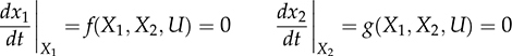
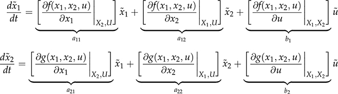

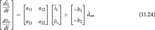
 represent the small signals; meanwhile, the values of X1, X2, and U are the steady-state equilibrium and become constant parameters. Thus, the state-space format can be formed by a group of the first-order differential equations
 or
or  is selected as the controlled output, y, according to the system specification, to form a transfer function,
  .
.
11.2 Linearization of Dual Active Bridge


 and
and  representing the output and input. The differential equation in (11.12) can be transformed into the s-domain transfer function as
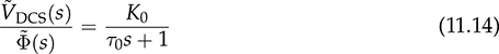
 and τ0 = REQCDCS. The output voltage shows the first-order dynamics in response to a small perturbation by the phase shift.
 ) is intentionally added to the steady-state phase shift angle (Φ), which is rated as ±2.5 mrad. For correct comparison, the offset of the equilibrium point should be added to match the waveform out of the large-signal model. The output of the small-signal model shows no information on the switching ripples but captures the critical dynamics in response to the step variation of
  in the small perturbation level. The first-order dynamic response is shown in Fig. 11.3, as predicted by the mathematical model in (11.14).
11.3 Linearization Based on CCM
11.3.1 Boost Converter
 and
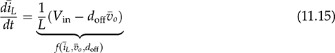
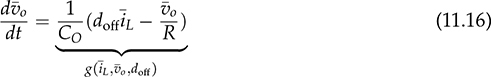
and  are nonlinear due to the multiplication of two variables. The model includes two state variables, which are the averaged values of inductor current and output voltage, shown as
 and
and  , respectively. The model input refers to the off-state duty, doff, which is doff = 1 − don in the CCM.
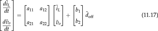


 and
and  ; meanwhile, the small-signal variation of the off-state duty ratio,
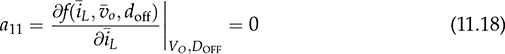
  , is the control input to the model. A more generalized model can be constructed by using
  instead of
  , since the on-state duty cycle, don, is commonly used as the control input. The small-signal model can be converted from (11.17) to (11.24), since the increment of on-state time is the decrement of the off-state in the CCM,
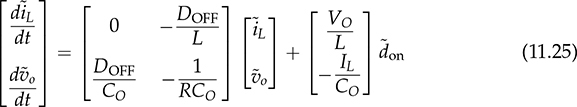
 , or the output voltage,
  , respectively. When
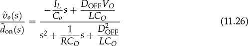
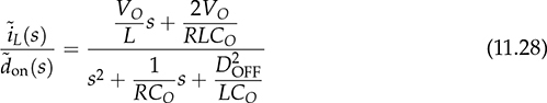
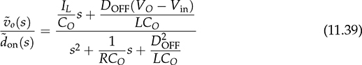
  is the interest for the dynamic analysis and control system design, a SISO transfer function in the s-domain can be derived from (11.25) into (11.26) or transferred to a generalized format in (11.27). A non-minimal-phase (NMP) zero is detected as
  , where βv > 0.


 and
and  . The transfer function shows the same denominator as G0v(s). The difference lies in the numerator sector showing the DC gain, K0i, and the minimal-phase zero, −1/βi.

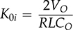
 and
and  . The zero in G0i(s) is −2667; negative value indicates the minimal-phase feature for the dynamic correspondence between
  and
and  . Figure 11.4 demonstrates the verification of the small-signal modeling. The time-domain simulation result is plotted and compared with the output of the large-scale switching model that has been developed in Chap. 3.

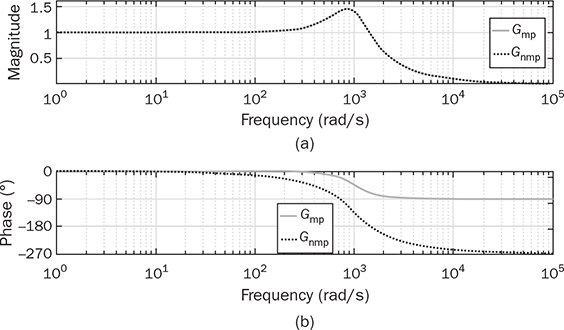
 = ±0.01, is applied to the nominal operating condition, where DON = 38.46% in the steady state. The steady-state values of the inductor current and output voltage have been derived as IL = 3 A and VO = 19.5 V, respectively. The increment of 1% at the moment of 20 ms and decrement of 1% at the moment of 30 ms lead to the transient response of iL and vo, as illustrated in Fig. 11.4. The steady-state values should be added to the small-signal model’s output to match the result of the large-scale model. The waveform agreement generally proves the effectiveness of the linearized models for analyzing the dynamics of boost converters. When a zoom-in is applied, the NMP effect is visible in the waveform of vo at the transient moment of 20 and 30 ms, as shown in Fig. 11.4. For comparison, the inductor current, iL, is also plotted, which does not show the NMP effect.
11.3.2 Buck-Boost Converter
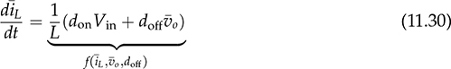
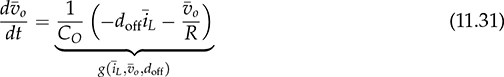
 and
and  symbolize the averaged value of the inductor current and output voltage, respectively. The model includes the nonlinear functions shown as f(
 ,
,  , doff) and g(
 ,
,  , doff) due to the multiplication of two variables, doff
 and doff
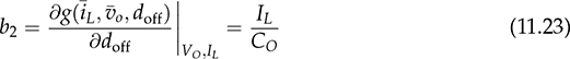
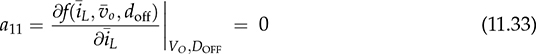
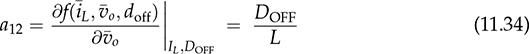
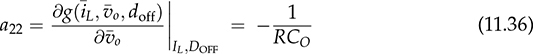
 . Applying the linearization process described in Sec. 11.1, the small-signal model for buck-boost converters can be derived into the state-space format:


 and
and  ; meanwhile, the small-signal variation of the on-state duty ratio,
  , is the control input to the model.
 or the output voltage
  , respectively. When
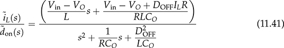
  is of interest for dynamic analysis and control system design, the transfer function in the s-domain can be derived from (11.32) into (11.39) or transferred to the generalized format in (11.40). A NMP zero can be detected in (11.40) as
  and βv > 0.

 and
and 

 and the value of βi can be accordingly determined.
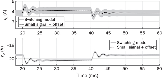
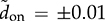 , is applied to the nominal operating condition, where DON = 52% in the steady state. Following the nominal operation and steady state, the averaged values of the inductor current and output voltage have been derived as IL = 3.85 A and VO = −19.5 V, respectively. The increment of 1% at the moment of 20 ms and decrement of 1% at the moment 40 ms lead to the transient response of iL and vo, as illustrated in Fig. 11.5. The steady-state values should be added to the small-signal model’s output to match the result of the large-scale model. The waveform agreement generally proves the effectiveness of the linearized models for analyzing the dynamics of the buck-boost converter. The NMP effect can be visualized by the zoom-in plot at the moment of 20 ms, as shown in Fig. 11.6. The effect is insignificant since the model reveals a fast NMP zero in the system dynamics.
11.3.3 Non-Minimal Phase
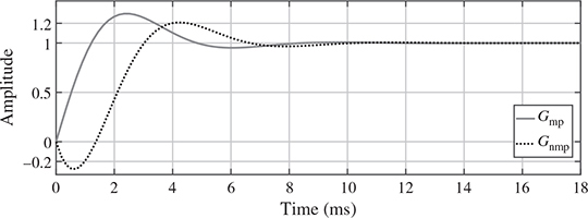
 and
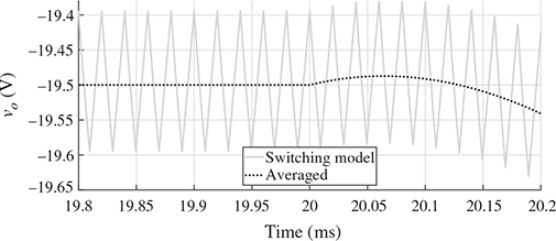
and  . The general form of a NMP transfer function, Gnmp, is defined and expressed in (11.43). The parameters of K0, ξ, and ωn follow the same definitions discussed earlier. The NMP zero can be found to be 1/β1, which is positive in value. For comparison, a minimal-phase (MP) transfer function is defined and expressed in (11.44), which follows the same parameters.


11.4 Linearization Based on DCM

 is the injected current, which symbolizes the average value of the inductor current for the buck converter. For the topologies of boost and buck-boost, the current value of
  represents the diode current. The transfer function can be derived to show the input-output relation between
  and
and  :
:
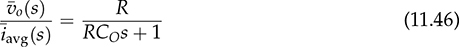
 and
and  . The speed of the first-order system depends on the values of CO and R.
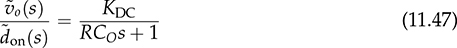
 by linearizing the voltage conversion ratio in (3.48). Accordingly, the gain value can be determined by other topologies. In general, when the DC/DC converter enters DCM, it presents the first-order dynamics, which is easy for analysis. The study in Sec. 10.4 has revealed the behavior of the first-order dynamics in the simulation results presented in Figs. 10.15, 10.17, and 10.19, for buck, boost, and buck-boost converters, respectively. The dynamic difference is noticeable during the transient states between the CCM and DCM. There is no overshoot or oscillation when the operation is switched from the CCM to the DCM.
11.5 Summary
Bibliography
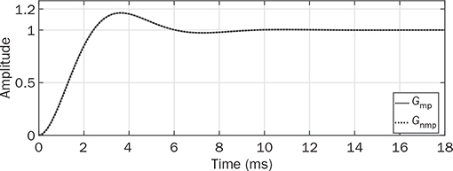
Problems
 and
and  in the CCM for the boost converter.
 and
and  in the CCM for the buckboost converter.