Abstract
In this chapter Maxwell’s equations are described and common ways to solve them analytically are discussed. The equations imply certain properties of matter with which it interacts and full solutions that describes this behavior analytically are provided from first principles. The chapter shows specifically that one can derive very fundamental properties with simple calculations. Furthermore, the concept of inductance and capacitance are highlighted by reference to their duality. Various high-speed phenomena are studied in some detail with particular attention to the current distributions induced by the magnetic field.
Learning Objectives
Maxwell’s equations in source form
Using estimation analysis in connection with Maxwell’s equations
Duality of capacitance vs inductance
One to three-dimensional solutions to Maxwell’s equations relevant to integrated circuit designers
Current distributions in various situations in order to estimate inductance
4.1 Introduction
This chapter discusses the basis of electromagnetism in terms of Maxwell’s equations. This topic that has been studied extensively and there are many great books that discuss its various aspects: see [1–14] for a small selection. Items [2, 5] focus on microwave aspects of the theory. Items [4, 8, 12] are standard physics graduate student texts. A more recent treatment is, for example [13, 14], which showcases engineering aspects of electromagnetism. We will follow the presentation in [1, 2] fairly closely. The intention in this chapter is to be self-consistent and in that spirit we will present common solution techniques found in the literature. The estimation techniques we discuss in this book will be heavily applied toward the end of the chapter where the concepts of capacitance and inductance are introduced. It is assumed that the reader has encountered electromagnetism before in elementary classes and we will not discuss the basic discoveries and the history that led to the remarkable formulation of the fundamental equations by Maxwell in a series of papers around 1865. The history of this development is a fascinating read and a great example of how science evolves [3].
We will start with a brief discussion of Maxwell’s equations and show how to reformulate them to be suitable in various situations encountered in integrated circuit design. Common solution techniques and handling of boundary conditions are presented next. Thereafter we will discuss the important concept of energy and power relating to the electromagnetic fields. These concepts will naturally lead to the definitions of capacitance and inductance both in general and for circuit theory. We will show that the concepts are naturally very similar, or dual, and we attempt to dispel some of the mystery that sometimes surrounds these phenomena. The chapter wraps up with a handful of examples where the estimation analysis technique is applied to calculate capacitance, inductance, skin effect, and other such effects. Most of these examples will start directly from Maxwell’s equations.
4.2 Maxwell’s Equations
This section presents Maxwell’s equations and we will follow the general outline presented in [1, 2]. Maxwell’s work was based on a large body of empirical and theoretical knowledge developed by Gauss, Ampere, Faraday, and others.
It is assumed that the reader has some familiarity with Maxwell’s equations and the history leading to their discovery. Here we will simply state them and highlight some of the historical events that surrounds them. The equations will be presented in their differential form. We believe most readers are familiar with the MKS or SI system of units and we will use them throughout the book.
With this we have for the equations:
 (4.1)
(4.1)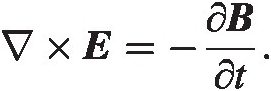 (4.3)
(4.3)
We have the quantities defined as:
HH is the magnetic field in amperes per meters [A/m]
DD is the electric flux density, in coulombs per meter squared [coul/m2]
JJ is the electric current density in amperes per meter squared [A/m2]
ρρ is the electric charge density in coulombs per meter cubed [coul/m3]
EE is the electric field in volts per meter [V/m]
BB is the magnetic flux density in webers per meter squared [Wb/m2]
The fields and their corresponding fluxes are related by the constitutional equations:
The factors ϵ, μϵ,μ are matrices in general and dependent on position. Throughout the book we will assume them to be scalar functions that are occasionally dependent on position.
Vector Potential and Elementary Gauge Theory
Having established Maxwell’s equations we can now take note of some interesting properties. For one, there are no magnetic charges, hence ∇ ⋅ B = 0∇⋅B=0. This means that instead of using BB we can define another entity AA by using the fact that for functions that are smooth, all derivatives exists and are continuous, we have the vector identity ∇ ⋅ (∇ × A) = 0∇⋅∇×A=0. This has important implications. If
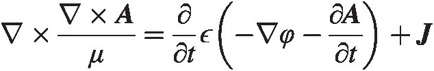
then equation (4.4) is automatically fulfilled. Substituting this into (4.3) we get
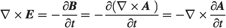
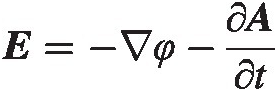
We now use the vector identity: ∇ × ∇ φ ≡ 0∇×∇φ≡0, where φ(x)φxt is any smooth function of coordinates xx and time t, to integrate EE and we find
 (4.8)
(4.8)The vector field AA is commonly referred to as the vector potential field and scalar φφ is known as the potential field, or voltage field. Together they are called gauge potentials in physics literature.
The equation for the EE-field should be familiar to most readers with the possible exception of the last term. Equation (4.8) is simply the normal elementary textbook definition of the electric field as a gradient of a voltage but with an additional time-derivative (dynamic) term. It means we can have an electric field without a voltage drop in a dynamic situation. With the potential fields we can write Maxwell’s equations to be a set of equations for φ and AφandA. Let us rewrite equation (4.1):
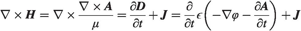
or
 (4.9)
(4.9)and from equations (4.2) and (4.5) we find
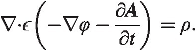 (4.10)
We now have another version of Maxwell’s equations through equations (4.7)–(4.10). As the reader will have noticed, the potentials, A, φA,φ are not uniquely defined. One can, for instance, add a term ~ ∇ f∼∇f where ff is some function to AA and the BB field is not affected (∇ × ∇ f ≡ 0)∇×∇f≡0. This freedom in the choice of the potentials is known as gauge invariance. Let us look at this in some more detail (compare with [15] for a similar argument).
Let γ(x, t)γxt be an arbitrary scalar field. Then let us change the gauge potentials according to the following transformation
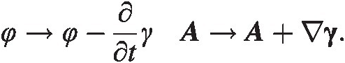 (4.11)
Now
and
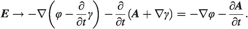
Both fields are unchanged! The transformation in equation (4.11) is known as a gauge transformation, and since the fields are unchanged under this transformation we speak of gauge symmetry. We see that a physical system is described by a whole family of gauge potentials that differ by a gauge transformation. By picking a particular set of gauge potentials we are making a gauge choice. The above might seem a trivial matter but it has profound importance in theoretical physics. The interested reader is highly encouraged to refer to the literature on this matter.
We will now show that we can always find a solution that satisfies
 (4.12)
by making an appropriate gauge choice. Assume we have a particular solution A′, φ′A′,φ′. We look for a particular gauge transformation that will satisfy (4.12). We have using (4.11)

or

The right-hand side is the known solution which acts as a source term for a wave equation which we can solve for γγ. This way we can always find gauge potentials that satisfy (4.12). We do not have to find γγ explicitly, but we can use this calculation as a motivation to use (4.12) as an additional requirement on A, φA,φ. Equation (4.12) is known as the Lorenz gauge. Another typical choice is the Coulomb gauge
The Lorenz gauge is typically used for situations where the wavelength is comparable to the physical sizes. It is standard in microwave theory and antenna theory for obvious reasons. For integrated circuits one can often get by with the Coulomb gauge which corresponds to the Lorenz gauge in the long-wavelength approximation.
Maxwell’s Equations in Terms of External Sources
In electrical engineering it is natural to think of currents and charges as being impressed on an electric system through voltage or current sources. These impressed entities will then give rise to electromagnetic fields. We will now write Maxwell’s equation in terms of such impressed currents and charges.
The current can be divided into two parts. A conduction component,
and an impressed current, JiJi. The charge can be divided the same way. By taking the divergence of equation (4.1) we recover the continuity equation:
 (4.15)
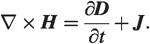
which relates the charge to the current. The addition of the time derivative of the DD-field to Ampere’s law (∇ × H = J)∇×H=J was Maxwell’s famous generalization that created a self-consistent description of the field equations. For the current we have

Putting this together we get
 (4.16)
 (4.17)
These equations show the fields as a result of external source currents and charges.
Full-Wave Approximation – Single Frequency Tone Formulation
In this book we will generally look at these equations not as a function of time but as a function of frequency. We get there by simply assuming the time dependence scales as ejωtejωt where we follow the convention in most engineering books. By doing this we get
 (4.18)
From the continuity equation for the conduction component we get
 (4.19)
This together with the charge equation (4.17) gives
 (4.20)
We can now define an effective permittivity
 (4.21)
and we have
Using equations (4.6)–(4.8) we get

We use the Lorenz gauge which in frequency domain looks like
and get
After rewriting we find
We also have from equation (4.23)

After rewriting we find
 (4.26)
Equations (4.25) and (4.26) are Maxwell’s equation in yet another form. Knowing A, φA,φ will give us B and EBandE through equations (4.7) and (4.8). We will use these in numerous examples in this and the following chapters.
Long Wavelength Approximation
In the long wavelength approximation, λ ≫ lλ≫l, where λ = 2πc/ωλ=2πc/ω is the wavelength and ll is a length scale of the model, we find the second term on the left-hand side of (4.25), (4.26) disappears and we are left with:
We can also write this directly from the fields as
where (4.27) follows if we use gauge ∇ ⋅ A = 0∇⋅A=0 and
 (4.29)
For integrated circuits the long wavelength approximation is often appropriate since the dimensions are much smaller than any wavelength.
Solutions to Maxwell’s Equations
Note the equations are of the same form where the only difference is the vector form for the vector potential and scalar from for the voltage field equation. The general solutions are known for certain sources. Here we will almost exclusively look at cases where the sources are Dirac delta functions of one sort or other. The specific solution will depend on the boundary conditions and most of the time will be spent establishing those.
For completeness, in this section we will discuss a common approach to solve wave style equations such as Maxwell’s. The first subsection covers the general solutions and we will discuss how to handle the all-important boundary conditions in the following subsection. We follow the presentation given in [1].
General Solution
We will start discussing the general solution of the one-dimensional case and follow with the two- and three-dimensional versions in the following subsections. There is a rich literature describing these methods and also a list of references at the end of the chapter.
1D – Solution
Let us consider an equation similar to (4.26) in free space
 (4.30)
This is known as Helmholz’s equation in one-dimensional free space subject to the boundary condition at infinity, φ(±∞) = 0φ±∞=0. The response at xx is due to the delta source at x0x0. Let us consider the homogeneous equation

This is the same as (4.30) when x ≠ x0x≠x0. The solution to this equation that satisfies the boundary conditions at infinity is

The unknown constants AA, BB can be determined by the boundary condition at x = x0 ± Δx=x0±Δ where ΔΔ denotes an infinitesimally small interval. Integrating (4.30) from x = x0 − Δx=x0−Δ to x = x0 + Δx=x0+Δ we find

Since φ(x)φx is continuous the last term on the left-hand side disappears when Δ → 0Δ→0.
We get

Solving for AA and BB gives
 (4.31)
Long Wavelength Approximation
When kx0 ≪ 1kx0≪1 (long wavelength approximation) we find

Since in the long wavelength approximation Helmholz equation reduces to Poisson equation where φlwφlw is defined with an arbitrary constant factor, we can simply relabel the constant term for φlwφlw and end up with
 (4.32)
Let us verify by examining the Poisson equation

When x ≠ x0x≠x0 we see ∂2φlwx∂x2≡0 . Let us integrate around the singularity as we did earlier

Indeed, in one dimension and the long wavelength approximation (4.32) solves the Poisson equation.
2D – Solution
In two dimensions equation (4.30) becomes
 (4.33)
We can now use the Fourier transform

This gives

The solution to this equation is the one-dimensional free-space Green’s function

where κ=k2−β2 . We find

where the last equality relates the Hankel function of order 0, H01 to the integral. We see the solution is simply a composition of a continuous spectrum of plane waves.
Long Wavelength Approximation
The two-dimensional solution in the long wavelength approximation can be found using similar techniques as in the one-dimensional case we noted earlier. Here we will show the solution for the special case of cylindrical symmetry which we will take advantage of later in this chapter when we discuss inductance and current elements.
Helmholz equation in cylindrical symmetry becomes, with a delta function at x = 0x=0,
Outside of x = 0x=0 we have

To further simplify we will assume there is no θθ-dependence and we find

This has the general solution
To find out the constants we need to integrate (4.34) around x = 0x=0. Let us choose a sphere centered at x = 0x=0 with radius ΔΔ as an integration volume. We find for the left-hand side using the divergence theorem (see Appendix B)

The right-hand side of (4.35) becomes, as before, CC. Putting all this together we have

We have for the long wavelength solution to the Helmholz equation in two dimensions:
 (4.35)
3D – Solution
We finally present the 3D solution. We will use it in Chapter 6. Equation (4.30) becomes with a source at r = r0r=r0

Let us first do a change of variables ρ = r − r0ρ=r−r0. We find we have created a spherically symmetric model. By realizing
we find

By substituting

we find for the Helmholz equation

The solution for u(ρ) = Aejkρuρ=Aejkρ and we find

The boundary condition at ρ = 0ρ=0 must be used to determine AA. The Helmholz equation is

After integrating over a small volume we find, as with the one-dimensional case,

After applying the divergence theorem we get

So

The general solution is

Similarly, for the vector potential we get

Long Wavelength Approximation
The solution to the long wavelength equations (4.27) and (4.29) in three dimensions are well known. We see the equations are essentially identical and the general solution that vanishes at infinity is
 (4.36)
The solution for φφ is similarly
 (4.37)
For a point charge at the origin, ρi(r′) = qδ(r′)ρir′=qδr′ we find

which is the familiar electrostatic potential from a point charge.
Boundary Conditions
Identifying the relevant equations and how to solve them is a helpful exercise. It is often the easiest part of any investigation. The real problem comes when taking into account what happens at the boundaries, either in time and/or in space. To the novice, the opposite often appears true. To help us there are many great examples in the literature on how to handle the boundaries, and here we will go through the basic methods and leave it to the reader to explore more if needed.
Fundamentally, what one does is to put a “pill box” at the boundary that extends a little into each material with a large surface area. In Figure 4.1 it extends ε/2ε/2 into each region. The volume is thus infinitesimal, while the area is macroscopic. They key thing to note here is that the equations are still valid in this volume and to find out what the boundary conditions are one simply integrates the equations over the small volume. For some entities, portions of the equation will be proportional to the volume and thus small while other entities will be proportional to the area and thus large. We will go through Maxwell’s equations with this method to show explicitly how the conditions work out.

Figure 4.1 Boundary conditions pill box.
Let us look at Ampere’s law (4.28)
At the boundary between two media we put a small pill box of height εε which is much smaller than any other dimension in the problem. We integrate Ampere’s law over this volume
We can here use Stoke’s theorem for the left-hand side and denoting by Area = AreanArea=Arean where AreaArea is the area and nn is the outward normal to the area segment
Volume Current
For the right-hand side without delta functions, which we call volume current, we get
Putting it all together we get at the boundary
or
Surface Current
We also see when we have a delta function on the right-hand side, a surface current,
Putting this together with the left-hand side we get
or
Similarly, we can use the charge equation (4.23)
We integrate over volume
For the left-hand side we use Gauss’ law

Volume Charge
For the case of volume charge, the right-hand side is now treated the same way as for the volume current earlier so we end up with
 (4.40)
Finally, for the case of surface charges we have

Field Energy Definitions
Let us look at the concept of energy in these fields. It is outside the scope of this book to fully derive this here but we will make some plausible arguments as to their validity: see [4] for details. Let us start with a static electric field where there are no currents.
Electric Field Energy
We assume for simplicity there is one conductor at a constant voltage φφ. If we have an infinitesimal charge δρδρ moving from infinity to the conductor we will need to apply an energy
Physicists like to call this entity “work,” but we will stick to using a less stringent definition of energy. We know from the boundary conditions, the charge on the conductor is
Here dSdS is a surface element and dSdS is surface element in the direction normal to the conductor surface. Since the potential is constant on the surface of the conductor we have
where in the last step we used Gauss’ law and the integral extends over all volume. Outside the conductor Maxwell’s equation states ∇ ⋅ δD = 0∇⋅δD=0. By expanding the integrand in the equation we see
We find
We can now substitute D = ϵED=ϵE and by looking at the integrand above

We have for the change in energy in the electric field

We can so make plausible the definition of energy contained in an electric field to be

Magnetic Field Energy
For a static magnetic field the situation is analogous. Here the work, or more roughly energy, done on currents is done by an electric field. A magnetic field by itself does no work on charges or current since it turns out that the magnetic force acting on a charge is perpendicular to its velocity. Instead we have to look for a situation where the magnetic field is varying with time, a quasi-static situation, and thus giving rise to an electric field through equation (4.3). We have in a time δtδt the energy spent by the external supplies
The first term can be transformed into a surface integral at infinity which we assume is zero, all fields vanish there. The second term we transform
As we did for the electric field, we again integrate the integrand

We get

We can now analogously to the electric field energy make plausible the definition of energy in a magnetic field

We now have
 (4.42)
The integral extends over the total volume. This is the time-dependent definition of the energies. In microwave theory the time average definition is more useful and we can simply get there by taking the time average assuming a sinusoidal wave. We get another factor of ½ for a total of ¼ times the volume integrals.
Capacitance: Definition
Let us assume we have a simple configuration of two conductors with a voltage φφ between them. We now define capacitance, CC, as
 (4.43)
In the general case we have

where in the last steps we used a common vector identity trick, ∇ ⋅ (φb) = b ⋅ ∇ φ + φ ∇ ⋅ b∇⋅φb=b⋅∇φ+φ∇⋅b. It has the convenient property that we only need to integrate over materials containing charges which greatly simplifies many calculations. By identifying terms we see capacitance is simply a linear relationship between charge and voltage. We will study this in more detail in the next section.
Key Concept
We need to know or estimate the voltages associated with various conductors and how the charge is distributed in order to estimate the capacitance.
Inductance: Definition
Analogously, for a simple situation with a wire carrying a current II, the inductance LL can be defined as
 (4.44)
For multiple currents JaJa we instead have the general formula

In previous steps we used a common trick to get rid of the large volume integrations by utilizing the vector identity: ∇ ⋅ (a × b) = b ⋅ ∇ × a − a ⋅ ∇ × b∇⋅a×b=b⋅∇×a−a⋅∇×b, and the divergence theorem coupled with the assumption the fields vanish at infinity. This shows we only need to integrate over materials where there is a current running. As we will see, this will greatly simplify some calculations.
If we calculate the contribution to AA from each current separately we can write

And we find
 (4.45)
where if a ≠ ba≠b we calculate the mutual inductance between elements a, ba,b and if a = ba=b we speak of self-inductance of element aa. We will use these facts later in this section.
Please note that when the vector potential from a certain conductor, say aa, is perpendicular to the current in another conductor bb the contribution from that term in (4.45) is zero. This is also an important simplification in many cases.
What the reader should take home from these calculations is the physical analogy between capacitance and inductance. One is based on voltage and charge the other on currents and vector potential. If you understand one of them you are likely to understand the other.
Key Concept
We know from elementary classes that currents will follow the least impedance path. In this context this simple rule means that the current will flow in way that minimizes inductance if there are no other effects like resistance/capacitance to consider.
We need to know or estimate how the currents are flowing in order to estimate the inductance.
The way to estimate inductance now becomes a way to estimate how the currents are flowing in the model. We will look at a number of situations where we will most of the time start directly from Maxwell’s equations and from there learn how the current distributes itself.
4.3 Capacitance
We have now finished with basic definitions of Maxwell’s equations and their solution and defined the concepts of capacitance and inductance. In the rest of the chapter we will apply the estimation analysis technique to explore these concepts more practically. We will find a way to simplify a given situation and we will solve and verify the solution. This will be followed by an evaluation phase. First we tackle something most likely very familiar to most engineers: capacitance.
Introduction
Most working engineers have a good feel what capacitance is and we will discuss it in ways that are very familiar with most readers and also use approaches that might not be as familiar but will prove to be good starting points and learning experiences. First we describe the circuit element: the capacitor. We then discuss a simple two plate system with a voltage between them which is an expansion of the discussion in section “Field Energy Definitions.” Thereafter we will solve the same problem using Maxwell’s equations directly where we also use the boundary conditions developed in section “Solutions to Maxwell’s Equations.” We will finally show how the same approach can be used when investigating an example with two different dielectrics.
Capacitors as a Circuit Element
So far we have discussed capacitance as it relates to physics: it is an effect that draws charge to a conductive surface when a voltage is applied to some other conductor. But what about capacitance as a circuit element? To investigate this we will use a simple conservation of power (or energy) argument. Imagine we have a resistor in parallel with a capacitor we know the power spent in the resistor is

where φφ is the voltage across the resistor and capacitor. The power in the capacitor is simply the time derivative of its energy

The voltage source that drives this combination is having a power φ(t) ∗ I(t)φt∗It pulled from it at a given time. This power has to equal the power spent in the resistor and capacitor:

or

This is the familiar circuit relationship. It becomes clearer if one assumes a time dependence ejωtejωt.

where the impedance due to capacitance is

We have shown the circuit formula for using capacitors follows simply from a conservation of energy argument.
Simple Two-Plate System Calculation
Let us use as a starting point equation (4.43). To get a feel for what these relationships mean in a real situation let us consider two metal plates of area AA, a distance, dd, from each other with a voltage φφ between them. The electric field is E = φ/dE=φ/d. We then have

or
 (4.47)
This is the normal calculation of capacitance known from elementary classes.
First Principle Calculation of Capacitance of Two-Plate System
Let us know look at the same situation from first principles, in this case Maxwell’s equations. We will follow the estimation analysis method. It will seem a little excessive at first, in particular when comparing with the previous calculation, but we will show we can easily extend what we learn here to other situations with little extra effort.
Simplify
The first thing to do is simplification. Let us imagine the two plates are infinitely extended in all directions in the plane. That will simplify the problem to one dimension. Next the top plate has a voltage, VV while the bottom plate is grounded. Lastly we assume the long wavelength approximation so we need to solve equation (4.26). We find as in Figure 4.2.

Figure 4.2 Two-dimensional projection of two plates.
In free space assuming no x-dependency we have then

Subject to the boundary conditions
Solve
This equation is independent of z and is a one-dimensional Helmholz equation in the long wavelength approximation which makes it Poisson’s equation and it has solution:
Let us plug in the boundary conditions


We get for
The electric field is E = − ∇ φE=−∇φ. At the lower perfect electrical conductor (PEC) boundary the electric field will change abruptly from the gradient of the potential to zero. This will result in surface charge and it follows from the boundary condition on ε ∇ ⋅ E = ρε∇⋅E=ρ which gives ϵE+ = ρϵE+=ρ. In effect what is happening is the voltage on the top is inducing a charge in the bottom plate. At long wavelength this is simply known as a capacitor effect. We will go through the simple derivation now.
We have

Since we now know the electric field we can simply plug it into the formula for capacitance (4.43) and recover equation (4.47). Going further we can use our more sophisticated model to recover another formula involving capacitance. Let us put a pill box around the boundary and integrating we find:

We have

where Q < 0Q<0. If we identify εy0Area=C or capacitance we have
This is another famous relationship involving capacitance and we see how straightforward it is to derive it directly from Maxwell’s equations.
Verify
This is the same result we saw earlier, leading to equation (4.47), but this was a more complicated calculation since we started from scratch. The advantage is we have learned a way to use Maxwell’s equations directly and we are now equipped to solve more complex problems.
Evaluate
The capacitance between two metal plates scales as the overlapping area of the plates divided by their distance.
First Principle Calculation of Capacitance with Two Different Dielectric Media
Here we will examine how the field solutions behave when there are different dielectric media in the problem. This situation often shows up in integrated circuits where there are different dielectric layers and instead of implementing all of them in a field solver it is often enough to use the equivalent permittivity. Here we will show how to calculate the effective permittivity and we will again start from Maxwell’s equations and end up with an expression that is quite familiar to most readers.
Simplify
We build on the previous simple model ad simply add another boundary: see Figure 4.3. All will still be one-dimensional.

Figure 4.3 Two-dimensional picture of two plates with two dielectric media.
Compared with previous calculations, everything is the same – the same equations, the same solutions – but we have an additional boundary condition at the interface between the two dielectrics. From ∇ ⋅ εE = ρ∇⋅εE=ρ we find
since there is no surface charge in the dielectric media.
Solve
We now have two region and two solutions:

For boundary conditions we get

The third one can be expanded:
or

We find from the fourth boundary condition

which gives

and

We find for the electric field at y = 0

As before we have for the charge at the lower PEC

We can rewrite this in more familiar form:

This is the well-known serial formula for capacitors. We can furthermore rewrite the equation in a form that makes use of an effective permittivity, ε′ε′

which gives

Verify
This is simply a rederivation of the well-known result of the equivalent capacitance of two capacitors in series. It is demonstrated in most elementary textbooks on electronics.
Evaluate
When stacking dielectrics with different permittivity the effective permittivity can be calculated as the inverse of a weighted sum of inverses.
Key Concept
When stacking dielectrics with different permittivity the effective permittivity can be calculated as the inverse of a weighted sum of inverses.
Summary
We have applied the estimation analysis to two situations where the total capacitance was needed. We calculated it directly from Maxwell’s equations using some basic simplifications as directed by the estimation analysis technique.
4.4 Inductance
We continue here with the concept of inductance. We have defined it in section “Field Energy Definitions” and we will here explore the definitions further looking at some simple situations where our estimation analysis technique will prove helpful.
Introduction
This section discusses the concept of inductance. As this concept may not be familiar to most engineers we hope to demystify it here. We will follow the outline in Section 4.3 to further show the analogy between inductance and capacitance, where we first discuss the circuit element – inductor – and then describe the simplest model followed by a treatment starting from Maxwell’s equations directly. Equipped with this we can attack more complicated problems. Much of the details here can be found in [4]. The inductance effect can be very detrimental to high-speed circuit behavior and one must understand its nature and how it can become large in order to produce successful designs.
Inductors as Circuit Elements
So far we have discussed inductors as it relates to physics: it is an effect that is proportional to the magnetic energy from a current distribution. It is not immediately obvious how it is related to circuit analysis. To investigate this we will use a simple conservation of power (or energy) argument.
Imagine we have a resistor in series with an inductor we know the power spent in the resistor is
where II is the current across the resistor and capacitor. The power in the inductor is simply the time derivative of its energy

The voltage source that drives this combination is having a power φ(t) ∗ I(t)φt∗It pulled from it at a given time. This power has to equal the power spent in the resistor and capacitor:

or

This is the familiar circuit relationship. It becomes clearer if one assume a time dependence ejωtejωt.
Where the impedance due to inductance is

We have shown the circuit formula for using inductors follows simply from a conservation of energy argument.
Simple Straight Wire in Free Space
We studied capacitance earlier in this chapter. Inductance is only slightly different. Instead of an electric field and charge, inductance relates to magnetic field and current. An electric field will look for other potentials on conductors around it to terminate, a magnetic field terminates on itself. This self-termination, which we will explore details below, can cause the magnetic field to become unbound. This has dramatic impact on the generating currents and how they can be allowed to behave.
Before we get into the mathematical details let us play a thought experiment. Imagine there is a universe with one unique feature: there is nothing in this universe but a wire, carrying a current, I. The wire is infinite and straight. We will assume Maxwell’s equations are valid. What is going on? Well, there is a current, so there must be a magnetic field (one of Maxwell’s laws). The converse is also true, if there is a magnetic field there has to be a current supporting it. The field stretches forever and ever around this wire. The total magnetic field energy,

What does this mean? If the magnetic field energy is infinite, so is the inductance. If you attempt to drive an AC current through this wire you will see an infinite impedance. In our simple universe, nothing can ever happen!
Admittedly this is far-fetched, but it serves to illustrate a point. In order for wires and currents to be useful there has to be a way to limit the far-field magnetic field. The way this is usually done is through loops either a current loop in itself or an induced return path in some ground plane. There has to be a closed current loop for circuitry to work! This is unlikely a surprise.
First Principle Calculation of a Simple Straight Wire
We will now dig deeper into the details of the previous section by starting from Maxwell’s equations directly using our estimation analysis.
Simplify
We have already set up a situation that is relatively simple. A straight wire in free space with uniform current distribution. We will model it as a system with no z-dependence, a two-dimensional system with cylindrical symmetry so all entities only depend on the distance, r, from the center of the wire. Seen from the side we find as in Figure 4.4.

Figure 4.4 Cross-section of single wire.
Let us look at this simple wire and dig into the mathematical details. We only need Ampere’s law in the long wavelength approximation
Solve
We can integrate Ampere’s law over a cross-section containing the wire as in Figure 4.5:
We can use Stoke’s theorem on the curl side:
where we have taken advantage of the cylindrical symmetry. On the right-hand side we get from the fact the current, JJ, is a density
Putting the two sides together we find

It is interesting to see here this result is independent of the precise radial distribution of the current internal to the conductor. The right-hand side is only sensitive to the total current in conductor.

Figure 4.5 Integration boundary of single wire.
Key Concept
The external magnetic field is not dependent on the radial current distribution inside the conductor in the cylindrically symmetric case.
This in turn implies that the inductance from the total magnetic energy is.

Here we have excluded the magnetic energy internal to the wire. It makes little difference. We find

where R is the “extent” of the wire. It has to be a closed loop somehow and RR is simply the size of the loop. We see the inductance will be infinite for a single wire without a loop as we hinted at in the previous section.
As a quick side note we can also calculate the vector potential outside the conductor when we know the magnetic field
 (4.49)
Evaluate
The inductance for a wire scales as the length of the wire times the logarithm of its size.
First Principle Calculation of Two Simple Straight Wires
Imagine now we have two wires where the current in one goes the opposite direction as the current in the other. The idea is to reduce the magnetic field in the single wire by creating an opposing field that is almost aligned. In effect we have a local current loop.
Simplify
We use the same basic model as previously but with the addition of one wire. The internal current distribution is assumed to be uniform: see Figure 4.6.

Solve
To calculate the inductance of the system we will use equation (4.46) we derived earlier. The equation states that knowing the vector potential and the current distribution inside the conductors we can calculate the inductance through a simple integration over the conductors cross-sections only. We have already assumed the current distribution is uniform and we are left with calculating the vector potential. The vector potential external to the wires we already know from equation (4.49). Let us also calculate AA inside a conductor. We have using the same strategy as in the previous section where we integrated Ampere’s law and used Stoke’s theorem:

where we have used the current density

and r ≤ R0r≤R0.
We get

From B = μH = ∇ × AB=μH=∇×A we find

where the constant has been chosen to match the external solution (4.49) at the r = R0r=R0 boundary. We can now put things together to calculate the energy by integrating the self-inductance and the mutual inductance from (4.46). We denote the energy for the self-inductance, FselfFself, and the energy for the mutual inductance calculation, FmutualFmutual.

where ZZ is the unit length of the wire. The variable r is the distance between the center of conductor 2 and r′, φ′r′,φ′ as indicated in the figure.
 (4.50)
The integral in the expression for FmutualFmutual can be calculated by identifying

This is straightforward to calculate and we find

Now
 (4.51)
The total energy is now

The other conductor combination is now easy to include because of symmetry, we just multiply by 2. By removing Jtotal2/2 we find the inductance is
 (4.52)
This is one of our fundamental results and we will use this again and again in various contexts.
Verify
This is a standard calculation in physics literature: see [4, 15], for example. For the reader coming from a microwave background this example might seem familiar. If so, it should, but the microwave literature often assumes the conductors to be ideal and in that case the solution is somewhat different. We leave it as an exercise for the reader to solve the ideal conductor case.
Evaluate
For two inductors on top of each other, if the current is going the same way in both inductors the magnetic field is doubled (with equal current) →→ magnetic energy is quadrupled →→ inductance is four times larger. If currents are going the opposite way →→ magnetic field is nulled →→ inductance is zero.
This effect is often referred to as coupling between the wires. It comes from the high frequency case where currents are induced in (or coupled to) the neighboring conductors.
Key Concept
For two inductors on top of each other, if the current is going the same way in both inductors the magnetic field is doubled (with equal current) →→ magnetic energy is quadrupled →→ inductance is four times larger. If currents are going the opposite way →→ magnetic field is nulled →→ inductance is zero.
This effect is often referred to as coupling between the wires. It comes from the high frequency case where currents are induced (or coupled to) in the neighboring conductors.
We will study the high frequency case and induced currents later in this chapter.
First Principle Calculation of Single Wire over Ground Plane
When a wire is running over a ground plane, we have a very similar situation to the previous discussion: see Figure 4.7.

Simplify
Using the method of images we can model the situation in exactly the same way where the distance dd is simply
where bb as in the figure is the distance to the ground plane from the wire. The method of images, [1], simply states the field outside a perfect ground plane can be found by removing the ground plane and put mirror conductors with opposite charge/current equidistant from the ground plane border.
Solve
We can now use exactly the same calculations as before with one important difference. The total field energy is now half of what we had before since no field exists in the ground plane which takes up half the volume.
We find
 (4.53)
Verify
This situation has been simulated as a 0.1 → 4 mm long wire (1 µm × 1 µm cross-section) over a ground plane in HFSS: see Figure 4.8.

Figure 4.8 Figure of an HFSS sim setup.
The conductor was a variable height over the ground plane. The excitation is through wave ports at the end of the structure as indicated. The inductance is calculated as

where YY refers to the Y-parameter (admittance) gain. Figure 4.9 shows the simulation comparison to (4.53) as a function of length where the height over the ground plane is 3 µm.

Figure 4.9 Simulated and estimated inductance of single wire over ground plane vs length.
A comparison of simulation vs estimation of inductance vs height over ground plane shows in Figure 4.10.

Figure 4.10 Inductance of single wire over ground plane vs height over ground plane.
Evaluate
When adding a ground plane under a conducting wire the resulting inductance will be reduced compared to a single wire. The inductance scales roughly as the logarithm of the distance to the ground plane. This is for the case of no other conductors nearby.
Key Concept
When adding a ground plane under a conducting wire the resulting inductance will be reduced compared to a single wire. The inductance scales roughly as the logarithm of the distance to the ground plane.
First Principle Calculation of a Current Sheet over a Ground Plane
Let us now look at the current analogue to a charge plane over a ground plane. This is the situation described in section “Simple Two-Plate System Calculation,” but now with a current sheet instead of a charge sheet (Figure 4.11).

Figure 4.11 Cross-section of current sheet over ground plane.
Simplify
Let us know look at the basic equations in terms of the vector potential A = A(y)ezA=Ayez, where the source term is a current. We could utilize the same simplifications we used in the capacitance calculation but here we will go one step further and start with the full wave equation and later go to the long wavelength limit so we can demonstrate some new mathematical steps.
In free space assuming no x-dependency we have
We have

Solve
We can use

This equation has the solution from equation (4.31).

For the boundary conditions we have
We get

From the boundary conditions we find:

Solving for the constant BB we get:

and

We have

At the long wavelength approximation we can simplify

By integrating the magnetic energy over the region we find:

From the definition of inductance, equation (4.4) we find
 (4.54)
The steps we followed here were more complicated than absolutely necessary to get to this answer. However, we have demonstrated a full solution to this version of Maxwell’s equations, in this case Helmholz equation, and we will look more into this kind of calculation in the rest of this chapter.
Verify
We can now see an interesting relationship with the calculation of capacitance between two plates. If we multiply equations (4.47) and (4.54):
 (4.55)
Evaluate
This turns out to be a general relationship for two dimensions, any two shapes have an inductance per unit length times a capacitance per unit length that is equal to μϵμϵ in two dimensions. The proof of this goes beyond the scope of this book but can be found in many references. It is a very useful rule to keep in mind. In practice it also holds up well for planar geometries in three dimensions where one has long skinny conductors. This is an example of a situation where estimation analysis yields a result that turns out to be quite general. If you find some simple relationship like the one just descrbied try to see if it is more general than your simplifications imply. Perhaps you have discovered something fundamental?
Key Concept
Any two shapes have an inductance per unit length times a capacitance per unit length that is equal to μϵ=1c2 for two dimensions. In three dimensions it holds well for planar geometries with long skinny conductors.
Summary
We have applied the estimation analysis to a few situations where the total inductance was needed. We calculated it directly from Maxwell’s equations using some basic simplifications as directed by the estimation analysis technique.
4.5 Various High Frequency Phenomena
Introduction
In this section we will study various high frequency phenomena that are of interest to the integrated circuit designer using estimation analysis. We will not consider frequencies so high the dielectric properties of the media changes. We will derive the skin depth phenomena from first principles in the first section. This will be followed by a study of induced current in a perfect ground plane, all from Maxwell’s equations or use solutions thereof studied earlier in this chapter. We will also study the general case of full wavelength approximation and how a resistive ground plane distributes its return current in the following section. We will finally see how currents in a thin metal wire, relevant to modern CMOS metal stack-ups, gets distributed.
Skin Depth
We have so far used the static approximation when studying inductance and come up with some useful approximations and concepts that will help us get a grip on the concept. Most of the time the wavelengths involved in IC design are large compared with the chip dimensions. However, there is one important exception due to the finite conductance in the routing layers giving rise to the “skin” effect. We will study this concept from the full Maxwell equations that will lead to some perhaps surprising results.
Simplify
We assume again cylindrical symmetry and we are using a spherical conductor with conductance σσ which we assume is high in the sense the effective permittivity is that of a good conductor: see Figure 4.12. Outside the conductor we assume again the long wavelength approximation since this is more common in circuit design. We have inside the conductor
Solve
Outside the conductor we have again

The magnetic flux density is

Inside the conductor the general solution is

representing an outgoing and an incoming wave. We will assume the outgoing wave is zero (E = 0)E=0. Above

With

We have

We find

We find for the solution

We see a term in the exponent of the solution that is real and shows a decline as a function of rr with a length scale
 (4.56)
Figure 4.12 Cross-section of single wire with a finite conductance.
Verify
This is known as the skin depth of the conductor.
Evaluate
The depth to which the electromagnetic fields can penetrate a conductor, skin depth, is dependent on frequency, conductivity and permeability according to (4.35). In typical small geometry CMOS processes the metal layers are really thin – 90 nm is not unusual. For a 6 GHz frequency in copper with a conductivity of 1.67 ∙ 10−810−8 ohmm we find a skin depth of 800 nm, 9× the thickness of some metal layers. So, when creating metal shields beware that there are enough metal layers stacked to make an efficient shield given the particular skin depth. Also, the resistance of the metal layers can be substantial – something to keep in mind for large currents.
Another interesting point here is the fact that when the skin depth is less than the conductor size the magnetic field is excluded from part of the conductor. Outside the conductor the field behaves independently of the current distribution inside the conductor and is not affected, as we noted earlier. This exclusion of the magnetic field thus lowers the total magnetic field over all space and the resulting inductance is reduced. This effect can be observed in simulators and while often not very big can reduce the inductance by a small percentage.
Key Concept
The depth to which the electromagnetic fields can penetrate a conductor, skin depth, is dependent on frequency, conductivity and permeability according to equation (4.56).
Currents Induced in Perfectly Conducting Ground Plane
We examined this situation previously in section “First Principle Calculation of Single Wire over Ground Plane.” We will here examine the induced current in the ground plane for this situation: see Figure 4.13. This calculation is important because it shows how one can estimate the current distributions in a more realistic situation. A good understanding of the current distribution is a key factor to understand inductance.

Figure 4.13 Current wire over infinite perfect ground plane.
Simplify
We examined this situation previously where we noted the resulting inductance is less when the ground plane is present. Here we will use the same approximations as before but we will look at the field solution near the ground plane. This situation is very common in the circuit world and it is worthwhile to explore this more.
Solve
The fields above the ground plane can be described as a sum of the field generated from the source current and a mirror field generated from a location equidistant from the ground plane but on the other side of the ground plane. The ground plane itself is removed. The phase of the mirror current is 180 degrees opposite the source current. This is known as the method of images and we described this earlier. We have from Figure 4.14:

At the ground plane we have from the boundary conditions that Hsum, x |y = 0Hsum,xy=0 is equal to the surface current in the ground plane. From symmetry we have r = r′r=r′ and we find from HH above

We see the induced ground current varies with a scale corresponding to the distance of the current above the ground plane: see Figure 4.15. This is as expected. Note that in this long wavelength approximation no other length scales exist with the exception of skin depth which here is zero. We explore this further in the next section.

Figure 4.14 Coordinate system of current over ground plane.

Figure 4.15 Current distribution plot.
Let us integrate this current density in the x-direction

so the total induced current is the same as the forced current. This makes sense since the magnetic field far away will then be canceled out by the two opposing currents.
Evaluate
The integrated induced current density is equal to the total imprinted current when no current loops are present. If this was not the case there would net magnetic fields at far distances and thus infinite impedance.
Key Concept
The integrated induced current density is equal to the total imprinted current when no other current loops are present.
Currents Induced in Resistive Ground Plane
When solving problems following the estimation analysis method it is not necessary to get an answer valid for all situations. Often it is very instructive to look at extreme points and from those behaviors draw conclusions about the full solution. Our next example will illustrate this point.
We have showed various approximations and how inductance can be derived and estimated depending on the geometry using various approximations that are helpful in integrated circuit design. We owe it to the reader to also present the full solution valid for any wavelength. This is also motivated by the rapid increase in extreme high-speed circuit development. Our discussion is similar to [1].
Simplify
Using the full Maxwell equations above we now assume with the same geometry as in Figure 4.13 but the perfect ground plane is replaced a resistive plane:
where JiJi is the impressed current. With the chosen coordinate system we find
We have
Solve
Since x is unbounded we can Fourier transform:

We have

We can just look at the integrand:

In general this equation cannot be solved exactly but needs a numerical solution.
For our case the solution has the general form:

With
Inside the lower material the solution is:

where

The boundary conditions are now

Also
We get

From Ez, BzEz,Bz is continuous we get

We see continuity of ByBy is guaranteed by the Ez = EzEz=Ez condition. Multiplying first by κ2κ2 and adding.

and

We have

The first term is the definition of Hankel function of degree zero:

Inside the lower material the solution is:
 (4.57)
This is a general solution and needs to be evaluated numerically for a given configuration.
Verify
However we can learn a few things by looking at extreme cases of key parameters. Let us use conductivity as such an example. Let us assume we have situation described in the previous section with static field and a ground plane with high conductance. We then have
or
The solution in media 2 is then

To get the current in the medium we need to take the curl of this twice. This corresponds to multiplying by −κ22 . In this extreme case we can limit ourselves to y = 0. So we find.

For high σσ we see the β2β2 will not dominate the sum for a long while. We can assume this happens when the first exponent |β| |y0|βy0 is very large so as to dampen out the integrand. We then get

This is a well-known Fourier inverse function and we have

We see we come back to our old solution, so this is encouraging. What about the other extreme where σσ is very small? We can still keep the long wavelength approximation both in medium 1, 2 and we find:

In the extreme case where σ = 0σ=0 we simply recover our old static solution where J = 0J=0 outside the current carrying conductor. What if σσ is simply really small so that when we look at the integrand that term containing σσ is only relevant for small ββ? By analogy with a more common physical situation where have frequency and time and not wavelength and distance we would say only the low frequency spectrum is affected and thus only long timescales will show any impact of σσ. Similarly, we can here say only long distances will show the impact of a situation where the conductivity is low. In other words, for high resistance substrates the current distribution under the current carrying conductor will be of the order 1/σωμ1/σωμ, which is large.
Evaluate
Although we have not provided a formal proof of the following Key Concept it is really just a reworking of Ohm’s law: More currents flow where the impedance is small.
Key Concept
In summary, the current in the plane under the signal will follow the path of lowest impedance. For high conductive substrates the dominant impedance is inductance and the current will be tightly distributed directly underneath the wire. For high resistance situations the current will spread out in the plane.
Current Distribution in Thin Conductors
Now that we have spent some time looking at various situations where inductance matters and we have learned the guiding principle is to have the currents flow in such a way as to lower the total magnetic energy, we will here investigate what will happen in a thin conducting slab where the thickness is smaller than the skin depth but the width of the wire is larger than the skin depth. Far away from the wire not much can be done, the generated magnetic field is not sensitive to the local distribution of the currents. But the near field is different and the currents will distribute themselves to sit near the short ends of the wire. This way the magnetic field in the symmetry plane through the conductor is zero and the total magnetic energy is smaller. We will quantify this fact in this section.
We will approach this problem using conformal transformations: see [17, 18]. It is a very powerful way to solve Laplace’s equation in two dimensions. It can be used not just in electrostatics but in many other physical fields.
This problem has been studied before in great detail: see [16]. We will not provide the exact solution since it is outside the scope of this book, but we will follow the estimation analysis approach we have been discussing.
Simplify
Let us consider the current distribution inside a metal slab. The general solution for a rectangular cross-section is difficult to solve analytically and has not been done to this author’s knowledge. However, for an ellipsoidal shape there is a known exact solution: [16]. Here we will just outline the model and do some simple scaling estimations to arrive at one of the asymptotic solutions. We will use the long wavelength approximation in two dimensions, with the current, JzJz, (and vector potential, AzAz) going in the z-direction, which states that externally we need to solve Laplace’s equation:
Imagine the conductor has the shape as described in Figure 4.16.

As a function of coordinates x, y the shape is described by

We will here go to the limit of h→0andσ→”large” such that h ≪ δ ≪ ah≪δ≪a and
For this situation we then naturally have the current in the slab is only dependent on xx.
Solve
We have from the definitions of the electric field in terms of the gauge potentials (4.49) and our assumption of Ez = 0Ez=0

Let us take the derivative w.r.t xx of the last expression. With our approximations we assume the only current flowing flows in the zz-direction. For this to be consistent the voltage drop along the segment in zz has to be constant over the surface of the conductor so we expect the derivative w.r.t xx to be zero.
 (4.60)
which becomes our boundary condition at the slab.
The problem amounts to solving Laplace’s equation for AzAz with the boundary condition (4.60) at the conductor. For large distances we must have from (4.49)
 (4.61)
corresponding to a current filament with a large return radius RR. This is our second boundary condition.
We now introduce the conformal coordinate transformation
yielding


The transformation is one-one with the restrictions
In the (x, y)-plane the curves of constant v are homofocal ellipses; the segment y = 0, |x| ≤ ay=0,x≤a is the infinitely flat ellipse v = 0v=0 and vv increases outwards to infinity: see Figure 4.17. The curves of constant u are the hyperbolae but there is a cut along the segment v = 0, so that u is positive in the upper-half plane Re y > 0Rey>0 and negative in the lower half-plane. The semi-infinite segment y = 0, x ≥ ay=0,x≥a corresponds to u = 0u=0, whereas the segment y = 0, x ≤ − ay=0,x≤−a corresponds to u = ± πu=±π.

With these new coordinates we have for our equation to solve
With the boundary conditions

The beauty of conformal transformations is if the solution solves Laplace’s equation in the new coordinates it also solves it in the old coordinates: see [17, 18]. The main advantage of this transformation is that if the new coordinates follow the basic geometry the equations are easier to solve.
We will further limit ourselves to the situation where u ≠ 0, ∓ πu≠0,∓π in other words we avoid the endpoints of the ellipsoid. We know the behavior of AzAz for large values of v and we also know when v → 0v→0 AzAz cannot have any dependence on xx (or uu in our new coordinates at the limit v → 0v→0). To meet Laplace’s equation we know a solution of the form
will work. To find C, BC,B we can attempt a look at the far distance requirement, v → ∞v→∞, equation (4.61) and see if we get a self-consistent solution. We have

Taking the logarithm of this we find

We can now identify the constants B, CB,C from (4.61) and (4.63) and we find
 (4.64)
This equation solves Laplace’s equation and as v → 0v→0 it has no dependence on uu which we need for the boundary condition at the slab and has the right scaling for large vv. In other words, it solves the conditions at the boundaries and the equation inside the domain. It is thus a solution to the problem. We will confirm this later when comparing to a more general solution.
We are interested in calculating the current across the thin slab with this solution. It can be calculated from the boundary condition discussed in section “Solutions to Maxwell’s Equations: Boundary Conditions,” in particular (4.39) where we here find
where Hx, 0Hx,0 refers to the size of the magnetic field at y = 0+y=0+. The magnetic field is given by (4.6) and (4.7).

We then find the current

And in terms of xx
 (4.66)
Verify
This problem has been solved more generally in [17]. The σ → ∞σ→∞ solution in that paper is the same as the one derived here. In the field solver we have analyzed the situation with various thicknesses. See Figure 4.18. As the thickness of the metal slab increase it is getting much better at expelling the field, just as we would expect from the simplified model. For thin wires the prediction fits reasonably well, within 10% except close to the end points (the actual edge is excluded because of the singularity in expression (4.66)). As the thickness increases the effect of the expulsion becomes clear and we see the skin depth start to dominate.


Figure 4.18 Simulation results and comparison wtih estimation analysis. The pictures to the left shows a cross section of the conductor with the current densities indicated in gray. The right pictures shows the current densities through the middle of the conductor. (a, b) corresponds to a thickness of 0.1 µm, (c, d) has a thickness of 0.5 µm, (e, f) shows a slab with 1 µm thickness, (g, h) has 2 µm thickness and finally (i, j) shows 5 µm thickness. The estimated curve has been normalized such that the current density in the middle of the conductor is the same for the simulated and estimated responses.
Evaluate
The lateral skin effect for wide conductors much thinner than the skin depth has a current length scale variation that is dependent on width only, equation (4.66). As the thickness increases the normal skin effect starts to manifest itself.
Key Concept
The lateral skin effect for wide conductors much thinner than the skin depth has a current length scale variation that is dependent on width only: equation (4.66).
4.6 Summary
In this chapter we have learned
We have defined Maxwell’s equations in a form that is useful for integrated circuit applications.
We have defined the physical concepts of inductance and capacitance.
To calculate capacitance the voltages need to be known
To calculate inductance, the currents need their direction to be known.
We have looked at various examples where we show how a given source current induces a current in neighboring inductors. Moreover, the current distribution within a conductor was derived for a number of examples. When neighboring conductors have significant resistive loss we found a version of ohms law that indicated how the current will distribute itself.
4.7 Exercises
1. Calculate the induced current in an isolated conductor from an outside current. Assume the outside current is fixed. Hint: a current sheet with a cylindrical isolated conductor could be a good starting point.
2. The total inductance in section “First Principle Calculation of Two Simple Straight Wires” was calculated assuming the current is evenly distributed inside the conductors. Calculate the inductance assuming the current only runs on the surface. Hint, if one calculates the capacitance the inductance is given by equation (4.55).
4.8 References
 Findit@CUHK Library | Google Scholar
 Findit@CUHK Library | Google Scholar
 Findit@CUHK Library | Google Scholar
 Findit@CUHK Library | Google Scholar
 Findit@CUHK Library | Google Scholar
 Findit@CUHK Library | Google Scholar
 Findit@CUHK Library | Google Scholar
 Findit@CUHK Library | Google Scholar
 Findit@CUHK Library | Google Scholar
 Findit@CUHK Library | Google Scholar
 Findit@CUHK Library | Google Scholar
 Findit@CUHK Library | Google Scholar
 Findit@CUHK Library | Google Scholar
 Findit@CUHK Library | Google Scholar
 Findit@CUHK Library | Google Scholar
 Findit@CUHK Library | Google Scholar
 Findit@CUHK Library | Google Scholar
 Findit@CUHK Library | Google Scholar