Simplify

We now make a number of simplifications:

• 
  

  The conductors are perfect, so no charge will penetrate into the volume of the conductors, i.e., they are surface charges.

  
  
• 
  

  We divide each conductor surface into much smaller surface segments where the charge is constant: see Figure 6.1.

  
  
• 
  

  There is only one dielectric medium, so no dielectric boundaries need to be considered.

  
  
• 
  

  We will ignore the complication of self-interaction where a given charge impacts the voltage on its own segment (there is a singularity). This is an important effect and not that difficult to deal with, but for illustrative purposes we will not address this problem here.

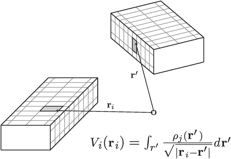
Figure 6.1 Conductors in three dimensions where the surface is divided up into smaller areas within which the charge is constant.

Solve

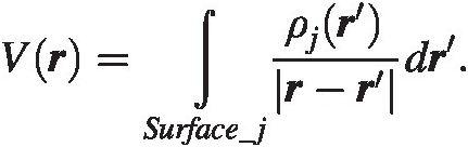
Let us now define the problem by looking at the potential from a charge on a surface segment jj, at a point rr. We have from equation (4.37)

Vr=∫Surface_jρjr′r−r’dr’.

We now calculate this voltage at a point in the center, r_iri, of another segment ii and sum over all segments. We find

Viri=∑j∫Surface_jρjr′ri−r’dr’=∑jρj∫Surface_j1ri−r’dr’.

This can be written as a matrix equation:

From the boundary condition we know the value of VV on all surfaces, and we can calculate GG and solve for ρρ. To get to capacitance, let us be a little more careful with notation. Let us assume we have N_segNseg conductor segments, each of which is subdivided into N_subNsub charge segments. We have a total number, N_tot = N_segN_subNtot=NsegNsub of charge segments. Let us denote by ρ_ijρij charge segment jj on conductor segment ii. In order to find the capacitance between conductor segment ii and jj, we need to ground all segments except ii, which has a voltage of V_i = VVi=V. We solve (6.1) and calculate the capacitance from (4.48)

Cij=1V∑k=1Nsubρjk.

With this procedure one needs to go through all conductors and set each voltage to VV one at a time, keeping all others grounded, solve the equation, and calculate the resulting capacitance. It sounds easy enough and it sort of is, but the difficulty lies in the details. The integrand has a divergence when i = ji=j that is fairly strong and the accuracy required in the numerical integration can be excessive. Furthermore, the grid is critical and in order to set it up properly one has to have a deep understanding of how charge will distribute itself on the surfaces beforehand. However, the pseudocode is straightforward.

Pseudocode

Subroutine build_G(Mesh)

                    * Loop over Mesh to build Matrix G.

                    For i = 0,N do

                              For j = 0,N do

                                        Integrate_element(r[i],r[j])

                              End for

                    End for

                    End build_G

                    Subroutine CapacitanceSolver

                    Create_mesh(Mesh)

                    G = Build_G(Mesh)

                    Ginv = Invert_matrix(G)

                    For i = 1,N do

                              V = Define_voltages(Mesh)

                              rho = Multiply(Ginv,V)

                              C[i] = sum(rho) // Assuming the voltage V = 1.

                    End for

                    End CapacitanceSolver

Verify

Simulators are traditionally verified by having them solve known problems and comparing the solutions. We leave it as an exercise to the reader to implement a code and gain experience by learning by actually doing.

Evaluate

We are not going to go to the trouble of actually building codes here, but simply state that although this may sound really simple and in some meaning of the word it is, the problem comes when you want accuracy. The charge tends to want to sit at the edges of the conductors, similar to the current distributions we examined in Chapter 5. This means that around those edges the surface elements must become really small to resolve the charge distribution, adding up to quite a few elements for large geometries. Some serious tricks need to be employed to get to the bottom of this and make the problem manageable. The most successful simulators have in common that they have found clever ways to manage the grid-generating algorithms. This has made some inventors very wealthy indeed. The construction of the grid and the speed with which the matric, GG, is calculated are critical parts of building simulators. If this is done poorly it will take a long time to find a solution for a given accuracy.

Simplify

We assume we are dealing with one long wire of a certain thickness and width that are much smaller than the conductor length. We chop the wire into small conductor segments where we assume several things:

• 
  

  The magnitude of the current in each conductor segment is the same, so there is no capacitive or other loss.

  
  
• 
  

  The current is uniform in a cross-section of the wire, in other words skin depth is not important. Each conductor segment can then cover the full cross-section of the wire.

  
  
• 
  

  These is only one magnetic medium, so no boundaries need to be considered.

  
  
• 
  

  We will ignore the complication of self-interaction where a given current segment impacts its own magnetic field (there is a singularity). This is an important effect and not that difficult to deal with, but for illustrative purposes we do not address this problem here.

Solve

Let us now define the problem by looking at the vector potential from a current on a conductor segment ii, at a point rr. We have from (4.36)

Air=∫Segment_iIir′r−r′dr′

With this expression we can now calculate the partial inductance matrix, L_{i, j}Li,j, between segments i,   ji,j, using (4.46) and

We find

Li,j=1IiIj∫Segment_jIjrj⋅Airjdrj=1IiIj∫Segment_jIjrj⋅∫Segment_iIirirj−ridridrj≈Ij⋅IiIiIj∫Segment_j∫Segment_i1rj−ridridrj=ej⋅ei∫Segment_j∫Segment_i1rj−ridridrj.

We refer to the case i ≠ ji≠j as the mutual inductance and i = ji=j as the self-inductance, similar to what we discussed earlier. Here we see explicitly the convenient fact that when the two currents are perpendicular to each other their mutual inductance is zero. If we decide not to divide the conductors – perhaps they are really thin, or frequency is low – we will be done here. We merely have to sum up all the elements to get the total inductance of the wire.

L=∑i,jLi,j

Notice the similarities in the expressions here compared with the previous section with the capacitance solver, where we summed over all charges and divided by the voltage difference to get the total capacitance between two conductors. There are a couple of important differences. For example, for the inductance case, we assume just one wire with a certain fixed current going through all segments. This greatly simplifies the analysis and we can just calculate the coupling without having to solve a matrix equation. The normal duality of capacitance and inductance is hidden due to these different assumptions.

But we can take this one step further and look at the situation where skin effect is important. We make some additional simplifications:

• 
  

  The conductors are close to ideal so the current will only flow within a certain surface depth. There is no resistive loss.

  
  
• 
  

  We divide the surface of each conductor segment into much smaller surface segments within which we assume the current is constant. For simplicity, the number of subsegments is the same for all conductor segments.

  
  
• 
  

  For a conductor segment, we assume the voltage drop across all surface segments is constant.

By subdividing the conductor segments into smaller segments where the current inside each is constant, we find similarly to before

Li,j=ei⋅ej∫Segment_j∫Segment_i1rj−ridridrj.

This defines the inductance matrix between each small surface segment. This is not quite what we want. We need the partial inductance for a particular conductor segment, which we can then sum up to find the total inductance of the whole structure, and we do not know the size of the current in each surface segment a priori. In order to move along we need to be a little more careful with the definition of the index notation. A surface segment, ii, belongs to a certain conductor kk and inside this conductor segment it has a subindex, ll. We then have the total number of current segments, N_totalNtotal is the total number of conductor segments, N_segNseg, times the total number of surface-segments, N_subNsub.

A particular current segment ii is then referred to as klkl. Likewise for the index jj we refer to a particular conductor segment mm and a subsegment nn (see Figure 6.2).

Figure 6.2 A cross-section of a conductor with subsegments where the mutual inductance integral is indicated.

We now know the partial inductance for each segment, and since we also know the total current we can calculate the voltage drop across each segment assuming a particular frequency ωω and using ohm’s law,

ΔVkl=jω∑m=1Nseg∑n=1NsubImnLkl,mn=∑m=1Nseg∑n=1NsubImnZkl,mn,

with Z_{kl, mn}Zkl,mn denoting the impedance matrix. This is just a matrix equation, and we can take the inverse to find the individual currents for each surface segment

Imn=∑k=1Nseg∑l=1NsubΔVklYmn,kl=∑k=1NsegΔVk∑l=1NsubYmn,kl,

where Y_{mn, kl}Ymn,kl is the admittance matrix. We start to see the resemblance to the capacitance calculation in section “Capacitance Simulations in Three Dimensions.” We can now take advantage of one of our simplifications, that the sum of all currents within a conductor segment is constant, conductor segment to conductor segment,

∑n=1NsubImn=I=constant.

We get

I=∑n=1NsubImn=∑k=1NsegΔVk∑n=1Nsub∑l=1NsubYmn,kl=∑k=1NsegΔVkym,k(6.2)

The matrix y_{m, k}ym,k is the admittance matrix between conductor segment mm and kk. After a simple inversion we find finally the impedance matrix between conductor segments.

And we can find the total inductance by

L=1jω∑i,jzij.

Pseudocode

Subroutine build_Zij(Mesh)

                    * Build Matrix by looping over the Mesh

                    For i = 0,N do

                             For j = 0,M do

                                        Integrate_element(r[i],r[j])

                             End for

                    End for

                    End build_Aij

                    Subroutine InductanceSolver

                    Create_mesh(Mesh)

                    Zij = Build_Zij(Mesh)

                    Yij = Matrix_Inverse(Zij)

                    yij = Contract_subsegments(Yij)

                    zij = Matrix_Inverse(yij)

                    End InductanceSolver

Verify

Reference [3] has a similar discussion but with more details.

Evaluate

Compared with the capacitance calculation, this is somewhat more complicated, and a few more steps need to be taken if the detailed surface current distribution needs to be known. However, the same caveats we listed in section “Capacitance Simulations in Three Dimensions” apply here. Building an efficient mesh, or grid, is challenging, since the currents tend to crowd near the edges as we outlined in Chapter 5, Figures 5.30 and 5.31. Another observation is that the duality we highlighted in Chapter 4 between capacitance and inductance is nontrivial to take advantage of, in that the capacitance calculation used the fact that the values of the potential, φφ, are known, and a fairly straightforward matrix equation can be set up. For the inductance case there is no boundary condition on the corresponding vector potential, AA. Instead, the boundary condition is set by the total current, so a few more steps need to be taken to solve for the inductance.

Delta Gap Source

A delta gap source is an impressed electric field between two conductors (see Figure 6.3). This field is then used as the external field in, for example, the method of moments. It is the simplest of the ports commonly used. For the integrated circuit designer it is quite relevant because of the small size of the active devices that connect to the conductors. For microwave applications it is much less common.

Figure 6.3 A simple 2D projection of two conductors with a field impressed between them. This is the incoming field and the way it is often pictured in the simulation setup.

Wave Port

A wave port is often defined on the boundaries of the system under consideration. Simply put, the fields are solved assuming two-dimensional symmetry on the boundary, as in Chapters 4 and 5. The intention is to mimic, say, a coaxial cable where there is an electromagnetic wave running, and it will look approximately like a field where the electric and magnetic field vectors are perpendicular to the direction of travel, hence the two-dimensional solution. Such a solution is then simply used as the boundary condition for the system under consideration. One can imagine modeling the input connector to a printed circuit board or some such application where this wave port model is a natural approximation. This type of port is very common in microwave applications.

Gaussian Elimination

With Gaussian elimination one simply reorders the equations through various multiplications/divisions and row additions/subtractions to end up with a single unknown in one of the equations, which can then be solved with simple back substitution. This is then solved and the process repeats with the now reduced set of equations. For more details see [2, 6]. This generally works but requires one to redo all the work for each rhs.

LU Decomposition

Here one eliminates the problem of the rhs by writing the matrix as a product of two other matrices, L,U such that A = LUA=LU. The LL matrix has the lower left triangle field including the diagonal, and UU has the upper right triangle field with zeros in the diagonal. This way of writing the equation results in another way of doing back substitution as earlier, but it no longer depends on the rhs, and as long as the matrix is not changing it is often a better method. References [2, 6] have more details.

Iterative Methods

What have really impacted the speed of the matrix inversion algorithms are iterative methods that can be very advantageous for large systems. The basic idea is to start with a guess, x₀x0 to the solution of Ax = bAx=b. The idea is to come up with a way to minimize the residual y = A(x − x₀)y=Ax−x0 by somehow calculating a new solution from x₁ = x₀ + βz₀x1=x0+βz0, where z₀z0 is some cleverly chosen direction. This goes on until the desired accuracy (size of |y|y) has been reached. There are a number of different ways of doing this, including conjugate gradient and biconjugate gradient methods (see [2, 6]). One class of remarkably easy to implement and efficient methods that work best for sparse matrices (frequently encountered in circuit systems) are the Krylov Subspace methods. See [7] for a good discussion on these techniques.